1. Introduction

In today's information age, predicting whether criminals are likely to commit crimes again has important practical significance and social value. By effectively predicting the risk of recidivism, preventive measures can be taken to reduce potential criminal behavior and protect public safety. It can not only improve the quality of judicial decision-making, optimize resource allocation, but also promote the rehabilitation of criminals, protect public safety, reduce the number of victims, and enhance the credibility of the judicial system. The decrease in recidivism rate means that society will face fewer criminal threats and ultimately establish a more harmonious and safe social environment. In the United States, the government uses risk assessment tools (RAI) to assist judges in determining who can be released on bail and who can be detained. The risk assessment process mainly relies on the dataset of criminal recidivism. These datasets typically contain various factors that affect crime (age, race, gender, etc.) as well as criminal history. Therefore, this article analyzes the factors that affect recidivism through existing datasets and constructs three models to predict recidivism rates and compare them. The model can classify prisoners as high-risk or medium risk, thereby helping judges determine sentencing measures for prisoners.

2. Literature review

The strongest predictor domains were criminogenic needs, criminal history/history of antisocial behavior, social achievement, age/gender/race, and family factors [1]. The widely used commercial risk assessment software COMPAS is no more accurate or fair than predictions made by people with little or no criminal justice expertise [2]. Recidivism prediction instruments (RPIs) provide decision-makers with an assessment of the likelihood that a criminal defendant will reoffend at a future point in time. Black defendants were far more likely than white defendants to be incorrectly judged to be at a higher risk of recidivism, while white defendants were more likely than black defendants to be incorrectly flagged as low risk [3]. This work ended up choosing the random forest model both to predict two-year recidivism and two-year violent recidivism. Our model for violent recidivism performs worse than our model for general recidivism; this is to be expected, however, considering the low prevalence of violent recidivism cases in the data. In both cases, the model slightly outperforms the corresponding COMPAS classifier. This work also gathered evidence that suggests that the COMPAS classifier is more biased against particular groups than our classifier [4]. In forecasting who would re-offend, the algorithm correctly predicted recidivism for black and white defendants at roughly the same rate (59 percent for white defendants, and 63 percent for black defendants) but made mistakes in very different ways [5].

3. Data exploration

3.1. Data acquisition

The dataset includes records of 6,172 individuals from Broward County, Florida, who have been convicted of a crime. The columns provided in the dataset include:

(1) number of prior convictions: The number of previous offenses or criminal convictions an individual has.

(2) age: The age of the indiviual at the time of the study or incident.

(3) gender: The gender of the individual, typically categorized as male, female,

(4) misdemeanor: A variable that might indicate whether the current or past offenses are misdemeanors (as opposed to felonies).

(5) ethnicity: The ethnic background of the individual, which may be used to study demographic trends.

(6) recidivism: A measure of whether the individual has reoffended after previous offenses, often within a specific period.

3.2. Data cleaning

The original dataset had 21 columns, but due to the presence of some duplicate data, duplicate columns or some almost worthless columns were removed. At the same time, categorical variables are converted to dummy variables, and transform variables with multiple categories into multiple dummy variables represented by 0 or 1. For example, dividing race into multiple dummy variables and dividing age into two dummy variables: young and old. Introducing dummy variables can help us solve the problem of multi class variables, enabling the model to better capture the impact of different classes on the dependent variable. This dataset has 6172 rows, and since there are no missing data, all rows of data have been retained.

3.3. Descriptive statistics

In this study, Exploratory Data Analysis was performed first to gain a comprehensive understanding of the dataset. The subsequent section provides a description of the data and the distributions for each variable.

3.3.1. Age groups

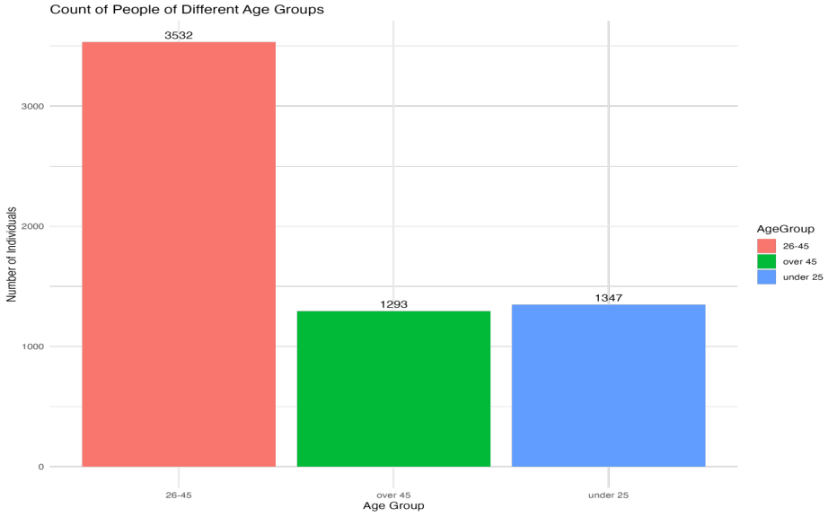
The analysis reveals a significant age-related pattern in criminal behavior. Most individuals involved in crime fall within the 26 to 45 age range, and about 20% of individuals engaged in criminal activities are either over 45 or under 25 years old as shown in Figure 1. This suggests that the likelihood of committing crimes is higher among people in the middle age group, whereas younger and older individuals are less prone to engage in criminal activities. Further exploration outside the current scope of analysis but potentially valuable for future research includes the impact of approaching significant age milestones on criminal behavior. Specifically, it would be insightful to investigate whether individuals nearing age milestones such as retirement show a higher propensity to commit crimes compared to their younger counterparts. This line of inquiry could provide deeper understanding of the social and psychological factors influencing criminal actions across different life stages.

3.3.2. Gender

As shown in Table 1, the gender variable is unevenly distributed between males and females. Men account for 81% of the total number of criminals, while women account for 19% of the total number of criminals. It can be seen that men are often more prone to committing crimes.

3.3.3. Ethnicity

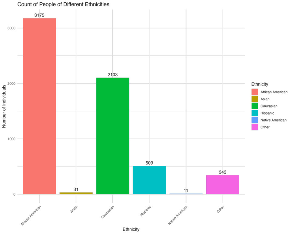
The analysis of the racial composition among the crime population reveals significant disparities. As shown in Figure 2, African Americans constitute approximately 50% of the total individuals involved in criminal activities, amounting to 3,175 people. Caucasians represent about 35% of the crime population, highlighting a pronounced involvement compared to other racial groups. In contrast, Native Americans and Asians each make up less than 1% of the total crime figures, indicating a much lower propensity for criminal involvement. Additionally, Hispanic and other racial groups collectively account for around 5%. These statistics suggest that race has a considerable influence on crime rates, with African Americans and Caucasians more likely to engage in criminal activities. This disparity raises important questions regarding the social, economic, and systemic factors that contribute to these observed patterns of criminal behavior across different racial groups. Further research could provide deeper insights into the mechanisms driving these disparities and help inform targeted interventions.

3.3.4. Charge degree

Table 2 shows that most people in the dataset (64%) have been charged with serious crimes, reaching 3970 individuals. 2202 people have been charged with minor offenses.

3.3.5. Descriptive statistics of reoffended prisoners

The analysis of recidivism within the dataset reveals that 2,809 prisoners have reoffended. Of these recidivists, a significant majority, 85%, are male, underscoring a strong gender disparity in repeat offending. Racially, African Americans and Caucasians together comprise 80% of the recidivism population, highlighting predominant trends among these groups. In terms of age, the 26 to 45 age bracket continues to represent a substantial portion of repeat offenders, like initial crime rates. However, there is a noticeable shift among younger individuals, who now constitute 27% of reoffenders, an increase from their representation in primary offenses. In contrast, only 15% of recidivists are elderly, suggesting a lower propensity for reoffending among older populations. Regarding the severity of crimes committed, data indicates that 71% of repeat offenses are committed by individuals previously convicted of serious crimes. This finding suggests a tendency for those who have engaged in severe criminal acts to reoffend, emphasizing the need for targeted interventions that specifically address the recidivism risks associated with serious offenses.

4. Methodology

4.1. Proposed model

In this study, four different machine learning models were used to predict the recidivism rate, namely Logistic Regression, Support Vector Machine, Decision Tree and Random Forest. This work divided the dataset into 80% training data and 20% test data. To fully analyze the predictive ability of these models in this context, each model is evaluated based on its performance on the test data with reference to four performance metrics, namely, accuracy, sensitivity, precision, and F1 score.

4.1.1. Logistic regression

Logistic regression extends linear regression to predict the probability of an event occurring by using the logit function to map the output to a range between 0 and 1, which allows it to be used to solve binary classification problems [6].

$$ P\left(y=1|X\right)=\frac{1}{1+e^{-\left({\beta }_0+{\beta }_1{x}_1+{\beta }_2{x}_2+\dots +{\beta }_n{x}_n\right)}}$$(1)

where  $$ \beta $$  represents the model coefficients and  $$ X$$  represents the features. The parameters of a Logit model,  $$ \beta =\left({\beta }_0,{\beta }_1,\dots ,{\beta }_k\right)$$ , are usually estimated by Maximum Likelihood Estimation (MLE). For ease of computation, the maximized log-likelihood function is generally computed. However, most of the time it does not have a closed-form solution, so it will be computed using gradient descent because in machine learning, the cost or loss function can be effectively minimized using gradient descent [7]. The gradient descent method iterates the parameters in such a way that they move in the direction of the steepest ascent of the log-likelihood function:

$$ {\beta }_{t+1}={\beta }_t+\alpha \nabla \mathcal{l}\left({\beta }_t\right)$$(2)

where  $$ \mathrm{\alpha }$$  is the learning rate, and  $$ \nabla \mathcal{l}\left({\beta }_t\right)$$  is the gradient of the log-likelihood function with respect to  $$ \beta $$  at the current iteration  $$ t$$ . The modeling process of logistic regression involves an iterative approach by trying to set up different combinations of variables as well as interaction terms and analyzing them with ANOVA and comparing their performance on test data. This resulted in a final logistic regression model with good performance and interpretability. The final model is shown below:

$logit(p_i)={\beta }_0+{\beta }^{\mathrm{T}}X+{ϵ}_i$(3)

where  $$ p_i$$  is the probability of reoffending for the  $$ \mathrm{i}$$ th individual,

$$ {\beta }^T=\left({\beta }_{\text{number\_of\_prior}},{ \beta }_{\text{male}},{ \beta }_{\text{old}},{ \beta }_{\text{young}}, {\beta }_{misden},{ \beta }_{\text{old:number\_of\_prior}},{ \beta }_{\text{young:number\_of\_prior}},{ \beta }_{\text{male:number\_of\_prior}}\right)$$(4)

$$ X={\left({\mathcal{x}}_{\text{number\_of\_priori}},{\mathcal{x}}_{\text{malei}},{\mathcal{x}}_{\text{oldi}},{\mathcal{x}}_{\text{youngi}}, {\mathcal{x}}_{\text{misdeni}},{\mathcal{x}}_{\text{old:number\_of\_priori}},{\mathcal{x}}_{\text{young:number\_of\_priori}},{\mathcal{x}}_{\text{male:number\_of\_priori}}\right)}^T$$(5)

4.1.2. Support vector machine

SVM is to find the optimal hyperplane in a high-dimensional space so that it splits the data points of different categories. To ensure the most efficient separation, SVM maximizes the margin, the distance between the hyperplane and the nearest data point in each category [8]. The method used in this study is the soft margins of the SVM, a method that allows for some misclassification, which weighs the margin width against the classification error, by introducing the slack variable  $$ {\xi }_i$$  and the cost parameter  $$ C$$ . The optimization problem is:

$$ \mathit{Minimize}: \frac{1}{2}{\Vert w\Vert }^2+C\sum _{i=1}^n{\xi }_i$$(6)

subject to  $$ y_i\left(w^T·\varphi \left(x_i\right)+b\right)\ge 1-{\xi }_i, {\xi }_i\ge 0$$ ,

where  $$ w$$  is the weight vector,  $$ b$$  is the bias. In this paper, a radial basis function kernel is used to find separating hyperplanes by mapping linearly non-separable data into a higher dimensional space, making it linearly separable [9].

$K(x,x\mathrm{\prime })=e^{-\gamma \text{‖}x-x\mathrm{\prime }{\text{‖}}^2}$(7)

Where  $$ {\Vert x-x\text{'}\Vert }^2$$  is the squared Euclidean distance between data points in the original feature space, the parameter  $$ \mathrm{\gamma }$$  controls the influence of a single training example. Based on previous exploratory analyses of the data, each variable could play a role in predicting recidivism, so all predictor variables were used to model the SVM to fully assess the impact of predictors on recidivism.

4.1.3. Decision tree

A decision tree is a tree-structured predictive model. The core idea is to recursively partition the data space, splitting it into increasingly smaller subsets until the subsets meet a stopping criterion. A decision tree consists of nodes and edges. Each node represents a feature, and each edge represents a possible value or range of that feature, thereby creating a structure that efficiently separates the data into distinct classes. Key components of this process include the use of entropy to measure the impurity of nodes, information gain to determine the most informative feature for each split [10], and cost complexity pruning to simplify the tree and prevent overfitting.

Entropy: A dataset's uncertainty or impurity is measured by entropy, which is used to evaluate the purity of a node. Entropy  $$ E\left(D\right)$$  for a dataset  $$ D$$  of binary classes can be mathematically represented as:

$$ E\left(D\right)=-p_{+}{\mathit{log}}_2\left(p_{+}\right)-p_{-}{\mathit{log}}_2\left(p_{-}\right)$$(8)

where  $$ {\mathrm{p}}_{+}$$  and  $$ {\mathrm{p}}_{-}$$  are the proportion of positive examples and negative examples in the set respectively.

Information Gain: The expected reduction in entropy is measured by Information Gain, which is utilized to determine the feature on which to split at each step in constructing the tree. The information gain  $$ IG\left(D,A\right)$$  for the dataset  $$ D$$  split on feature  $$ A$$  is:

$$ IG\left(D,A\right)=E\left(D\right)-\sum _{v\in Values\left(A\right)}\frac{\left|D_v\right|}{\left|D\right|}E\left(D_v\right)$$(9)

where  $$ D_v$$  is the subset of  $$ D$$  where feature  $$ A$$  has value  $$ v$$ .

Cost Complexity Pruning: Cost complexity pruning is a method utilized to streamline a decision tree by cutting away branches that hold minimal significance.

The tree is pruned using a complexity parameter  $$ \alpha $$  that controls the trade-off between the tree's complexity and its accuracy [11]. The cost complexity is calculated as:

$$ R_{\alpha }\left(T\right)=R\left(T\right)+\alpha \times \left|Leaves\left(T\right)\right|$$(10)

where  $$ R\left(T\right)$$  is the misclassification rate of the tree, and  $$ \left|Leaves\left(T\right)\right|$$  is the number of nodes. This work constructed the decision tree model by analyzing the relationships among key variables, including the number of prior convictions, age (young and old), gender and dummy variables of race. To prevent overfitting, the work optimized the model using cost complexity pruning, which helped simplify the model's structure. In the final pruned model, the number of prior convictions, age, and gender were identified as the primary factors influencing recidivism risk. Figure 3 shows how the final decision tree model performs the classification task.

4.1.4. Random forest

Random Forest, an ensemble technique, enhances model accuracy and robustness by aggregating multiple decision trees. In the process of building each decision tree, Random Forest randomly chooses a subset of features from the entire set, promoting diversity among the trees. Then, each tree makes an independent prediction, and the final prediction is determined by majority vote. By random feature selection and voting mechanism, Random Forest effectively reduces overfitting and offers better generalization to new data. The final model uses various predictors such as the number of prior convictions, demographic factors (age groups and male), the type of current offense and ethnicity dummies. Then the hyperparameter setup is like this, 500 trees are grown in the forest, which helps ensure that the model is stable and less prone to overfitting. The number of variables at each split is approximately 3, the square root of the number of predictors. Although the random forest model has strong predictive power, its characteristics make it less explanatory as a model for predicting recidivism.

4.2. Performance metrics

The classification models constructed during the implementation phase were evaluated using key performance metrics, including accuracy, sensitivity (recall), precision, and the F1 score. These metrics provide a comprehensive assessment of the models' ability to correctly predict whether an individual was likely to reoffend within two years of their current offense. Table 3 shows the confusion matrix and the definitions of true negative (TN), false negative (FN), true positive (TP), false positive (FP).

4.2.1. Accuracy

Accuracy measures the overall prediction capability of the model. In the context of recidivism prediction, a high accuracy indicates that the model can correctly predict whether an individual will re-offend in most cases.

$$ Accuracy=\frac{TP+TN}{TP+TN+FP+FN}$$(11)

4.2.2. Sensitivity (recall)

Sensitivity, also known as recall, is used here to assess whether the model can correctly identify most people who will reoffend. It refers to the proportion of true positive predictions relative to the total number of actual positive cases.

$$ Sensitivity=\frac{TP}{TP+FN}$$(12)

4.2.3. Precision

Precision is used to assess whether most people predicted to reoffend are true reoffenders. It is calculated as the ratio of true positive predictions to all positive predictions made by the model.

$$ Precision=\frac{TP}{TP+FP}$$(13)

4.2.4. F1 score

The F1 score, the reconciled mean of precision and recall, is used to model whether the model can both effectively identify actual re-offenders and simultaneously minimize false alarms.

$$ F1 Score=\frac{2\times Recall\times Precision}{Recall+Precision}$$(14)

5. Results

This work compares the performance of four different models in predicting recidivism rates. These models are Logistic Regression, Support Vector Machine, Decision Tree, and Random Forest. The work uses four evaluation metrics: Accuracy, Sensitivity, Precision, and F1 Score to conduct the comparison and analysis. The results are showed in Table 4.

According to Table 4, the Logistic Regression model has an accuracy of 0.687, the highest among the four models, indicating that it has the best overall prediction capability. This means that the Logistic Regression model can correctly predict whether an individual will re-offend in most cases. Its sensitivity is 0.665, also the highest, showing that it is quite good at identifying most of the individuals who will actually re-offend. However, its precision is only 0.577, the second lowest among the models, indicating that a significant portion of those predicted to re-offend are false positives. The F1 score is 0.618, balancing sensitivity and precision, but it is lower due to the low precision.

The Support Vector Machine model has an accuracy of 0.669 base on Table 4, slightly lower than Logistic Regression, but still relatively high. Its sensitivity is 0.647, the third highest, meaning it is somewhat less effective at identifying true positives compared to Logistic Regression and Random Forest. The precision is 0.536, lower than other three models, indicating more false positives. The F1 score is 0.586, still be the lowest, indicating a bad performance affected by lower precision.

The Table 4 shows that the Decision Tree model has an accuracy of 0.667, the lowest among the four models, suggesting it is the least effective in overall prediction. Its sensitivity is 0.606, the lowest, indicating it struggles the most with identifying actual re-offenders. However, the Decision Tree model has the highest precision of 0.686, suggesting it has the fewest false positives. The F1 score is 0.644, the highest among the models, indicating it maintains the best balance between precision and sensitivity. The Random Forest model has an accuracy of 0.679, medium performance, shows that the prediction ability of the model is moderate. Its sensitivity is 0.649, the second highest, showing it effectively identifies individuals who will re-offend. The precision is 0.584, the second highest, indicating a good rate of true positive predictions. The F1 score is 0.615, close to Logistic Regression, showing it balances precision and sensitivity well.

6. Conclusion

The result indicate that Each model has its own advantages and limitations. In logistic regression, each feature has a corresponding coefficient, and these coefficients directly determine the influence of the feature on the probability of the predicted outcome. The positive coefficient indicates the positive correlation between the feature and the result, and the negative coefficient indicates the negative correlation. Moreover, logistic regression is usually based on the maximum likelihood estimate for parameter estimation, and the maximum likelihood estimate itself is resistant to outliers, so the logistic regression model is relatively robust. So logistic regression is suitable for those cases in need of transparency and robustness. According to the test, logistic regression model has the best performance in accuracy and sensitivity, indicating that it has strong ability in prediction accuracy and coverage, and is suitable for those situations requiring broad identification of potential recidivism. However, low in accuracy means that the model may generate more false positives, which can be a disadvantage in some applications that are sensitive to false positives.

The idea of SVM is to find an optimal hyperplane (a straight line in two-dimensional space, a plane or hyperplane in higher dimensional space) so that different classes of data have the greatest spacing on both sides of this hyperplane. This maximum interval characteristic makes SVM have better generalization ability and reduces the risk of overfitting. In this test, the overall performance of support vector machines is relatively bad across all models, especially in accuracy and F1 scores. And that suggests that if the situation don’t accept the high cost of miscalculation, caution should be exercised in choosing this model. The decision tree considers only one feature at a time of segmentation, it can flexibly adapt to the way different features affect the output variables. This single-feature focus strategy, combined with recursive segmentation, enables decision trees to effectively deal with non-linear features. Also, decision trees usually do not require normalization or standardization of the data. They can process raw data directly and are insensitive to different scales of data. In this test, decision tree is good at precision, which makes it the best model for reducing false positives. It is still an option worth considering if the goal is to minimize the recurrence of misidentification, although its performance in accuracy and sensitivity is not optimal.

The random forest is an integrated model composed of multiple decision trees. While a single decision tree is very interpretive because each decision point and path can be visually seen, a random forest contains many such trees, each of which may give different predictions, and the final prediction is based on the combined results of all the trees. This integration process makes the model decision complex and non-transparent. In this test, the random forest model shows a good balance, and its performance is more balanced in every index. This feature makes random forest the most suitable option in cases where both false positives and missed positives need to be considered. In conclusion, while Logistic Regression has the best accuracy and sensitivity, the Decision Tree model provides the best balance between precision and sensitivity, making it a strong candidate for predicting recidivism with fewer false positives. However, the final choice of the model should also consider the specific requirements and constraints of the prediction task.

References

[1]. Chouldechova, A. (2017).Fair prediction with disparate impact: A study of bias in recidivism prediction instruments. Big Data., 5(2): 153–163.
[2]. Dressel, J., & Farid, H. (2018). The accuracy, fairness, and limits of predicting recidivism. Science Advances., 4(1): eaao5580.
[3]. Gendreau, P., Little, T., & Goggin, C. (1996) A meta-analysis of the predictors of adult offender recidivism: What works! Criminology., 34(4): 575–608.
[4]. Hayes, B. (2018) Predicting criminal recidivism with R. https: //benhay.es/posts/predicting-criminal-recidivism-r/#top
[5]. Jeff, L., & Surya, M., & Lauren, K. (2016) How do we analyze the COMPAS recidivism algorithm. https: //www.propublica.org/article/how-we-analyzed-the-compas-recidivism-algorithm
[6]. Hosmer, D. W., & Lemeshow, S. (2000) Applied logistic regression (2nd ed.). Wiley. ISBN 978-0-471-35632-5.
[7]. Boyd, S., & Vandenberghe, L. (2004) Convex optimization. Cambridge University Press. ISBN 978-0-521-83378-3.
[8]. Cortes, C., & Vapnik, V. (1995) Support-vector networks. Machine Learning., 20(3): 273–297.
[9]. Awad, M., & Khanna, R. (2015) Support vector machines for classification. In Efficient learning machines. pp. 39–66.
[10]. Krishnan, S. (2021) Decision tree for classification: Entropy and information gain. Medium. https: //medium.com/codex/decision-tree-for-classification-entropy-and-information-gain-cd9f99a26e0d
[11]. Pennsylvania State University. (n.d.) 11.8.2 - Assessing the adequacy of the model | STAT 508. Online Learning, Penn State. https: //online.stat.psu.edu/stat508/lesson/11/11.8/11.8.2
Cite this article
Wang,R.;Gu,Z.;Su,Q. (2025). Comparative Analysis of Machine Learning Models in Predicting Recidivism. Advances in Economics, Management and Political Sciences,213,65-75.
Data availability
The datasets used and/or analyzed during the current study will be available from the authors upon reasonable request.
Disclaimer/Publisher's Note
The statements, opinions and data contained in all publications are solely those of the individual author(s) and contributor(s) and not of EWA Publishing and/or the editor(s). EWA Publishing and/or the editor(s) disclaim responsibility for any injury to people or property resulting from any ideas, methods, instructions or products referred to in the content.
About volume
Volume title: Proceedings of the 4th International Conference on Financial Technology and Business Analysis
© 2024 by the author(s). Licensee EWA Publishing, Oxford, UK. This article is an open access article distributed under the terms and
conditions of the Creative Commons Attribution (CC BY) license. Authors who
publish this series agree to the following terms:
1. Authors retain copyright and grant the series right of first publication with the work simultaneously licensed under a Creative Commons
Attribution License that allows others to share the work with an acknowledgment of the work's authorship and initial publication in this
series.
2. Authors are able to enter into separate, additional contractual arrangements for the non-exclusive distribution of the series's published
version of the work (e.g., post it to an institutional repository or publish it in a book), with an acknowledgment of its initial
publication in this series.
3. Authors are permitted and encouraged to post their work online (e.g., in institutional repositories or on their website) prior to and
during the submission process, as it can lead to productive exchanges, as well as earlier and greater citation of published work (See
Open access policy for details).