1. Introduction

The transfer market, where soccer clubs all over the world invest a huge amount of money to hire or release players in the transfer window period every summer and winter [1], is a crucial part of the world’s professional soccer system. Transfer fees, a key part of this market, refers to the money that one club pays another to get a player's registration. A player’s transfer market value, an estimate of the value of the player to clubs provided by transfermarkt.de [2], is commonly used as a starting point for talks, but his actual transfer fee is usually different. In recent years, players’ transfer fees have been rising, including the highest one, Neymar to Paris SG in 2017, for 220 million EUR [3]. However, current performance measures may not capture the full picture of a player’s value, and the key factors behind the gap between market value and actual transfer fees are not fully understood. Therefore, clubs, agents, and analysts who work in this high-stakes environment need to know what influences a player's market value and what distinguishes the actual transfer fee from the market value, in order to better determine the clauses included in the contract to maximize their own profit.

English Premier League (PL), is one of the richest and most competitive soccer leagues in the world. After Season 24/25, the PL rank 1^st among all the associations and leagues in Europe with a total UEFA score of 90.839, which is 9.893 higher than the second place, Italy [4]. Also, Merten proved that there is a significant positive correlation between transfer spending and league ranking [5]. Therefore, PL clubs’ transfer market activities attract the attention across the world, leading to enormous personnel and currency flows. This study aims to examine the main factors that affect the prices of player transfers with statistical analyses of PL club data, in order to get a better understanding of the complicated transfer system and promote research in sports economics, statistics, and market behavior.

2. Data & methodology

2.1. Examining the factors that influence players’ market value

Used in real market transactions and wage negotiations and able to predict actual transfer fees [6], market value can be influenced by many different factors. The authors hypothesize that the main factors influencing a player’s market value are his age, position and on-field performance. This study collected all PL players’ names, ages, positions, market value, and market value change in Season 24/25 from the website Transfermarkt [7], and the players’ performance scores from average Sofascore ratings in Season 24/25 [8].

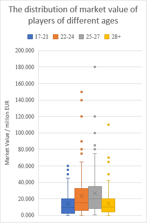
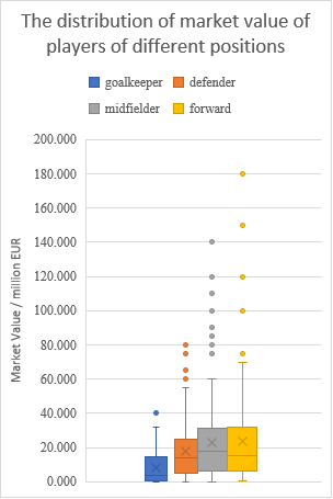
First, all the 616 players in the PL are divided into 4 age groups with similar populations: 136 players under 21, 158 players aged from 22 to 24, 161 players aged from 25 to 27, and 161 players over 28. A box plot is created to compare the mean, median, range and outliers of the players’ market value in different age groups. Second, another box plot is created to examine the influence of players’ positions on their market value. The players are also divided into 4 groups: 68 goalkeepers, 205 defenders, 176 midfielders and 167 forwards. Thus, the authors are able to compare the distribution of market value of players of different positions. Third, the authors applied two ANOVA tests to quantitatively examine the means of players’ market value in different age and position groups.

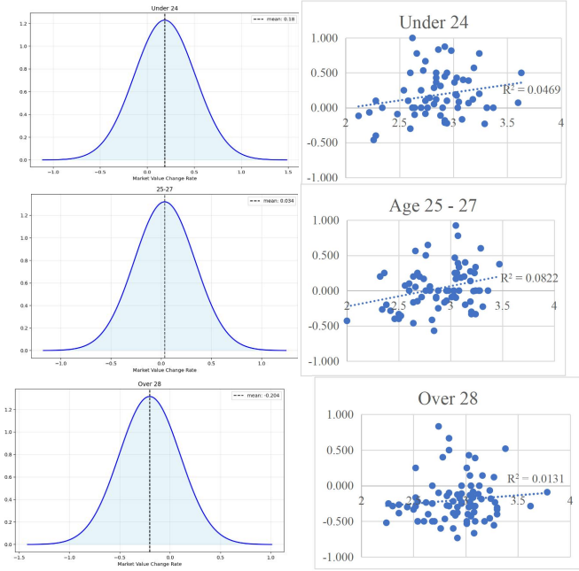
Then, three scatterplots are generated with their x-values representing players performance score and their y-values representing players’ market value change rate. The scatterplots present data of players under 24 years old, age from 25 to 27, and over 28, respectively, in order to eliminate the effects of players’ ages on their market value change. The performance score is calculated based on Sofascore ratings of players who have at least 15 appearances with more than 10 minutes on field in PL in Season 24/25 in the following way: Sofascore ratings range from 3.00 to 10.00, which is divided into 6 intervals, [3,6), [6,6.5), [6.5,7), [7,8), [8,9) and [9,10]. Since most PL players’ average ratings are between 6.00 and 8.00, the 3.00 rating is transferred to 0 and 10.00 is transferred to 6, while each interval is equally divided into 100 parts which are each transferred to 0.01, in order to amplify the difference between players’ performance scores. Outliers with market value change rates over 100% are eliminated in the scatterplots. Moreover, three normal distribution curves are generated based on the mean and standard deviation of the market value change rate in the 3 age groups, in order to examine the influence of age on players’ market value change.

2.2. Examining the factors that distinguish players’ transfer fees from their market value

For most of the transfers, the players’ transfer fees are usually different from their market value. Poli et al. recognized that 'market value is only proxy for player wages or transfer fees’, and that 'there are conceptual differences between market values and transfer fees’ [9]. The authors hypothesized that the expire time of players’ original contracts is an important factor that leads to the difference. In other words, there might be a significant distinction between the transfer fees of players who are in the last year of their contract and players who are not.

The authors collected the data, including the market value, transfer fees and the year in which the players’ original contracts are going to expire, of players who joined or left the Big 6 clubs from Season 23/24 to Season 25/26 with both their market value and transfer fee over 10 million EUR. Loans, free transfers and players who haven’t signed a professional contract or whose contract details are not open to public are excluded. The authors calculated the rate of difference between transfer fees and market value in the following way and excludes the transfers where the difference rates are larger than 1:

$$$ difference rate=\frac{\left( transfer fee- market value \right)}{market value}$$$

Then the remaining 62 transfers are divided into 2 categories, 13 players who are in the last year of their contract and 49 players who are not. Thus, data in the 2 categories can be seen as two sample, and by calculating their mean and standard deviation, 3 t-tests can be carried out in order to tell whether the expire time of players’ original contracts will distinguish players’ transfer fees from their market value: 2 one-sample t-tests for population mean to examine whether the population mean of the 2 samples are significantly larger or smaller than 0, respectively, and a 2-sample t-test for a difference between population means to compare the distributions of the difference rate between the 2 kinds of players.

3. Empirical results

3.1. Data analyses of factors that influence players’ market value

Players range from 17 to 39 years old, with a mean age of approximately 25.5 years (based on prior calculations). The sample skews younger, reflecting soccer's emphasis on youth development, with peaks around 22-26 years. According to Figure 1, players aged from 22 to 24 and from 25 to 27, with the largest outlier of 180 million EUR, have higher mean and median than the other groups, indicating that these players, who are on the rise or at their peak, are more likely to have a higher market value. In contrast, players under 21, who just entered the professional league, and players over 28, whose careers are on the decline and about to end in a few years, often have a lower market value. This indicates that a player’s market value is likely to rise when they are under 24, fluctuate when they are aged between 25 to 27, and fall when they are over 28. Also, goalkeepers and defenders, who usually do not engage in attacks and goals, have a significantly lower mean and median in market value, with no outliers above 80 million EUR; however, midfielders and forwards, with 8 outliers above 100 million EUR, have a higher market value in general. This shows a greater market attention towards players who have the ability to attack and score than those who play a defensive role in the modern soccer system.

Then two ANOVA tests are applied, one for different age groups and the other for position groups, as shown in Table 1 and Table 2. According to Table 1, a p-value less than 0.001 in the ANOVA Table shows that there are significant differences between the population mean of market value of players in different age groups. Moreover, p-values in the Tukey HSD for age group table indicates that there is no significant difference between the mean of players aged over 28 and that of players under 21, as well as the two groups of players who aged from 22 to 24 and from 25 to 27; in contrast, players aged from 22 to 24 and from 25 to 27 have a significantly higher population mean in market value than players aged over 28 and under 21 in the other 4 groups of comparisons. Therefore, age-wise, values surge during the 22-27 prime years, driven by peak performance and resale prospects, before plummeting post-28 due to injury risks and career twilight.

According to Table 2, a p-value less than 0.001 in the ANOVA Table shows that there are significant differences between the population mean of the market value of players from different positions. Moreover, p-values in the Tukey HSD for position group table indicates that there is no significant difference between the mean of midfielders and forwards; in contrast, goalkeepers show a significantly lower population mean in all 3 comparisons, while defenders are proved to have a lower population than midfielders and forwards at a confidence level of 0.10, but not at 0.05. Therefore, the findings underscore a market bias toward offensive contributions, as forwards and midfielders fetch premiums for goal-scoring potential.

In Figure 2, the scatterplots and R²-values indicate that, performance ratings will positively influence players’ market value change rate to a small extent, since the regression lines all have slightly positive slopes; but there is only a weak correlation between market value change rate and performance ratings because of low goodness of fit. This implies that performance probably works as a minor factor that only influences players’ market value in a small degree. By analyzing the mean and standard deviation of the samples and generating normal distribution curves, players under 24 have a mean of 18.5% increase in market value with a standard deviation of 32.5%, indicating that a player under 24 years old will have a predicted probability of 71.5% to have an increase in market value; in contrast, players over 28 have a mean of 20.4% decrease in market value with a standard deviation of 30.3%, indicating that a player over 28 years old will have a predicted probability of 74.8% to have a decrease in market value. This obvious pattern proves that age works as a more significant factor than performance that influences players’ market value change rate.

3.2. Data analyses of factors that distinguish players’ transfer fees from their market value

The authors used 3 pieces of python code to do the 3 t-tests, two one-sample t-tests for population mean and a two-sample t-test for a difference between population means. The outputs are shown respectively in Table 3, Table 4 and Table 5.

In the first one-sample t-test for population mean, the null hypothesis is that the population mean inferred from Sample 1 equals to 0, while the alternative hypothesis is that μ will be less than 0. According to Table 3, Sample 1, which consists of players in the last year of their contrasts, shows a mean value of -0.092 and a standard deviation of 0.224 in the difference rate between their transfer fees and their market value. The t-test generates a t-statistic of -1.474 and a p-value of 0.083, indicating that the null hypothesis will be rejected at a confidence level of 0.10, but will not be rejected at a confidence level of 0.05. Therefore, at a confidence level of 0.10, the population mean of the difference rate between the transfer fees and the market value of players who are in the last year of their contracts is predicted to be less than 0.

In the second one-sample t-test for population mean, the null hypothesis is that the population mean inferred from Sample 2 equals to 0, while the alternative hypothesis is that μ will be greater than 0. According to Table 4, Sample 2, which consists of players who are not in the last year of their contrasts, shows a mean value of 0.132 and a standard deviation of 0.312 in the difference rate between their transfer fees and their market value. The t-test generates a t-statistic of 2.962 and a p-value of 0.002, indicating that the null hypothesis will be rejected at a confidence level of 0.05. Therefore, at a confidence level of 0.05, the population mean of the difference rate between the transfer fees and the market value of players who are not in the last year of their contracts is predicted to be greater than 0.

In the two-sample t-test for a difference between population means, the null hypothesis is that there is no difference between the population means. According to Table 5, the t-test shows a t-statistic of -2.924 and a p-value of 0.007, indicating that the null hypothesis is rejected at a confidence level of 0.05. Therefore, the population mean inferred from Sample 1 is significantly lower than the one inferred from Sample 2.

In conclusion, the difference rate between market value and transfer fee of a player who are in the last year of their contrast is likely to be less than that of players who are not, the former less than 0 and the latter greater than 0 in general.

4. Conclusion & discussion

4.1. Factors that influence players’ market value

In the previous parts, the authors identified age and position as main factors influencing players’ market value. According to the data analyses, players aged between 22 and 27 are more likely to have higher market values, showing the preference of clubs for players who are on the rise or at their peak of their career; forwards and midfielders have an obviously higher average market value than defenders and goalkeepers, indicating clubs’ greater attention towards players who take an offensive role. This pattern informs club strategies, favoring investments in young attackers for financial upside, amid evolving transfer dynamics.

Of all age groups, linear regression model demonstrates that performance ratings will positively influence players’ market value change rate to a small extent. However, the R²-value of the groups are all below 0.10, which proves a weak correlation between market value change rate and performance ratings, indicating that the linear regression model might not be the best method to examine the relationship between players’ performance and their market value change rate. Also, the Sofascore Rating might not be a proper representative of the players’ performance; to improve the result, further researches can use different indicators to measure the performance of players in different positions, such as goals for forwards and saves for goalkeepers. This method might meet the problem of not getting a sufficient sample size, but this can be solved by expanding the data from the Premier League to the Big 5 Leagues, including the Premier League, Ligue 1 in France, La Liga in Spain, Bundesliga in Germany, and Serie A in Italy.

4.2. Factors that distinguish players’ transfer fees from their market value

The authors identified that players whose original contracts have only one year remaining will have a transfer fee significantly lower than others, the former usually having a transfer fee lower than market value and the latter being the opposite. Accordingly, clubs should target contract-expiring players to control their expenditure and avoid trading players away in the last year of their contracts to lower their losses. However, the sample size of Sample 1 is 13, which is too small and might cause the one-sample t-test for population mean to be biased, probably exaggerating the probability of Type I Error, in other words, mistakenly rejecting a true H0. Also, the unequal sample size in the two-sample t-test for a difference between population mean, 13 in Sample 1 and 49 in Sample 2, might also increase the probability of making Type I or II Errors, while a Welch’s t-test may be able to solve this problem. Moreover, there are 2 possible causes of the relatively small sample size: the study is limited to Premier League and the BIG 6 clubs, and the data of some transfers is not open to the public. Therefore, future researches can expand the data to more clubs in various leagues in order to get a sample large enough for a more reliable conclusion.

Future researches can also focus on other potential factors that cannot be examined from the data in this study: for example, whether competition between different clubs or exposure to social media will influence a players transfer fee.

4.3. Clubs’ operations to increase transfer revenue or control expenditure

The financial status of clubs is not negligible when they determine how much they’ll pay for a player. Franceschi et al. recognized that 'the buying club’s bargaining power seems to show evidence of influencing the valuation of player’ [10]. Under the restrict of the Financial Fair Play, which consists of 2 major provisions – the no overdue payables rule and the break-even rule [11] – “many clubs depend on incomes generated on the transfer market to balance their books” [9]. In other words, the revenue of a club determines the budget it is able to put on the transfer market. Therefore, clubs will try to use different kinds of operations to lower their expenditures on players they buy or raise their revenue from players they trade.

First, some operations are directly related to the transfer fee. By applying payment with installments, for example, clubs can spread the cost of a player over the entire contract term [12], in order to reduce the immediate expenses on a single player and thus be able to spend more money in the transfer window.

Second, clubs may choose to trigger the buyout clauses, which 'permit a player or another club to pay a stipulated sum in the contract and effectively terminate the agreement, irrespective of its stipulated duration’ [13]. In this way, if the penalties for triggering the clause is lower than the player’s market value, buyer clubs will not have to meet the requirements of the seller club, lowering its expenditures on trading for a player.

Third, additional clauses might be inserted in transfer contracts between clubs, including sell-on clauses, through which 'the selling club, against a lower immediate transfer fee, retains the right to a certain percentage of a potential future transfer fee of the player to a third club’ [14]. This clause is often applied on young players who are considered promising when they transferred to other clubs, thus their original club can still earn a profit from their future development.

Acknowledgments

Siqi Zhou and Donghan Li contributed equally to this work and should be considered co-first authors.

References

[1]. Behravan, I., & Razavi, S. M. (2021). A novel machine learning method for estimating football players’ value in the transfer market. Soft Computing, 25(3), 2499-2511.
[2]. Coates, D., & Parshakov, P. (2022). The wisdom of crowds and transfer market values. European Journal of Operational Research, 301(2), 523-534.
[3]. Metelski, A. (2021). Factors affecting the value of football players in the transfer market. Journal of Physical Education and Sport, 21, 1150-1155.
[4]. UEFA. (2025). Country coefficients | UEFA ranking. https: //www.uefa.com/nationalassociations/uefarankings/country/?year=2026
[5]. Merten B. (2022). The Impact of Transfer Spending in Expediting Improvement of On-Field Performance of English Premier League Clubs.
[6]. Herm, S., Callsen-Bracker, H. M., & Kreis, H. (2014). When the crowd evaluates soccer players’ market values: Accuracy and evaluation attributes of an online community. Sport Management Review, 17(4), 484-492.
[7]. Transfermarkt. (2025). Premier League 25/26 | Transfermarkt. https: //www.transfermarkt.com/premier-league/startseite/wettbewerb/GB1
[8]. Sofascore. (2025). Premier League 2024/2025 table, schedule & stats | Sofascore. https: //www.sofascore.com/tournament/football/england/premier-league/17#id: 76986
[9]. Poli, R., Besson, R., & Ravenel, L. (2021). Econometric approach to assessing the transfer fees and values of professional football players. Economies, 10(1), 4.
[10]. Franceschi, M., Brocard, J. F., Follert, F., & Gouguet, J. J. (2024). Determinants of football players’ valuation: A systematic review. Journal of Economic Surveys, 38(3), 577-600.
[11]. Plumley, D., Ramchandani, G. M., & Wilson, R. (2019). The unintended consequence of Financial Fair Play: An examination of competitive balance across five European football leagues. Sport, Business and Management: An International Journal, 9(2), 118-133.
[12]. Ciliberto, F., Scotti, D., & Vismara, S. (2025). The Market for Player Rights: Trading and Price Manipulation in European Soccer, 2015-2023. Available at SSRN 5375621.
[13]. Giancaspro, M. (2016). Buy-out clauses in professional football player contracts: questions of legality and integrity. The International Sports Law Journal, 16(1), 22-36.
[14]. Colantuoni, L., & Devlies, W. A. (2016). The Sell-on Clause in Football: Recent Cases and Evolutions. In Yearbook of International Sports Arbitration 2015 (pp. 73-91). The Hague: TMC Asser Press.
Cite this article
Zhou,S.;Li,D. (2025). Examining the Factors That Influence Players’ Transfer Fees in English Premier League. Advances in Economics, Management and Political Sciences,218,129-137.
Data availability
The datasets used and/or analyzed during the current study will be available from the authors upon reasonable request.
Disclaimer/Publisher's Note
The statements, opinions and data contained in all publications are solely those of the individual author(s) and contributor(s) and not of EWA Publishing and/or the editor(s). EWA Publishing and/or the editor(s) disclaim responsibility for any injury to people or property resulting from any ideas, methods, instructions or products referred to in the content.
About volume
Volume title: Proceedings of ICEMGD 2025 Symposium: Resilient Business Strategies in Global Markets
© 2024 by the author(s). Licensee EWA Publishing, Oxford, UK. This article is an open access article distributed under the terms and
conditions of the Creative Commons Attribution (CC BY) license. Authors who
publish this series agree to the following terms:
1. Authors retain copyright and grant the series right of first publication with the work simultaneously licensed under a Creative Commons
Attribution License that allows others to share the work with an acknowledgment of the work's authorship and initial publication in this
series.
2. Authors are able to enter into separate, additional contractual arrangements for the non-exclusive distribution of the series's published
version of the work (e.g., post it to an institutional repository or publish it in a book), with an acknowledgment of its initial
publication in this series.
3. Authors are permitted and encouraged to post their work online (e.g., in institutional repositories or on their website) prior to and
during the submission process, as it can lead to productive exchanges, as well as earlier and greater citation of published work (See
Open access policy for details).