1.  Introduction

The index model developed by William Sharpe in 1963 remains one of the most widely utilized financial portfolio construction models until this day, despite the subsequent development of more sophisticated multi-factor frameworks. More advanced and accurate models such as the Three Factor Fama and French Model, and the Five Factor Fama and French Model were developed and ameliorated the explanatory power by incorporating factors such as market risk, size, value, profitability, and investment [1]. Empirical research has consistently validated the advancements of these multi-factor models. For example, Chiah, Chai, and Zhong verified the superiority of the Five Factor Fama French Model over the Three Factor model by demonstrating its ability to explain more pricing anomalies [2]. In response to the growing number of models, Fama and French also provided further guidance on using the maximum squared Sharpe ratio as a way of measuring model efficacy [3]. Research by Ye, Wang, and Raza has further explored the maximum attainable Sharpe ratio under different constraints [4]. The utility of the Index Model for optimization purposes has also been a focus of study, as examined by Mistry and Khatwani [5].

Despite these advancements, the Single Index Model retains significant relevance for educational and practical applications. This study leverages its streamlined framework to investigate how portfolio optimization behaves under different constraints. The portfolios to be examined will be constructed of the S&P 500 index and 21 constituent stocks, spanning five major sectors. Comparisons will be made on the results produced by the index model under the unconstrained ("Free") and constrained ("Box" constraint, where |w_i| ≤ 1) scenarios, to simulate a realistic case.

The goal of this analysis is to empirically verify fundamental portfolio theories, such as the trade-off between risk and return and the impact of constraints on the efficient frontier; and to provide a hands-on, practical perspective that complements textbook treatments for investors and future researchers. By bridging theoretical models with real-world applications, this study aims to enhance understanding of how constraints shape investment outcomes and portfolio efficiency.

2.  Data and model

2.1.  Data

2.1.1.  Stock selection

The portfolios constructed in this paper will be based on the S&P 500 Index and 21 constituent stocks (table 1) from five different sectors, including Financial, Industrial, Technology, and Basic Materials. To mimic a realistic investor portfolio, this study selected industry leaders among the most popular stocks.

2.1.2.  Data processing 

This study used 20 years of daily data (September 2004 to September 2024) obtained from OEX Bloomberg for each of the selected securities and performed a series of processing to extract useful information for portfolio construction.

As the Central Limit Theorem suggests, data of aggregated financial returns depict normality due to aggregational Gaussianity [6]. For verification, the distribution graphs of daily returns and monthly returns have been plotted, and the results are consistent with the theory. Thus, for the sake of accuracy, assumptions of the model used, and simplicity of calculations, the data will be aggregated into monthly data. This process is done through Excel by taking out the securities’ prices at the end of each month, utilizing the filter function.

The next step is to find the relevant values required to perform calculations of the index model, given the monthly prices of the selected securities, which include the annualized average excess return of the S&P 500 index  $$ E\left(R_M\right)$$ , the S&P 500 Index standard deviation  $$ {\sigma }_M$$ , Beta (  $$ {\beta }_i)$$ , Annualized Alpha ( $$ {\alpha }_i$$ ), and Annualized firm-specific risk  $$ {\sigma }_{}^2\left(e_i\right)$$ .

It is worth noting that the equation for the Index model is based on excess return; thus, the data must be adjusted accordingly. To achieve this, this study relies on estimating a set of values of the notional risk-free rate (NRFR) based on the Fed Funds Effective Rate (FEDL01) using the following function, with the first period of FEDL01 set to be 1000 for simplicity of calculations. Where the 100 is used to convert the value of FEDL01 to a percentage, and 261 is the number of trading days within a year.

$$ {NRFR}_{n+1}={NRFR}_n\star (1+FEDL01)/100/261$$(1)

The monthly return for each security was calculated first by dividing the security’s price in the current month by its price in the previous month, minus one. The monthly excess return for each of the securities is then computed as the monthly return minus NRFR. Annualized Average Excess Return of the S&P 500 Index  $$ E\left(R_M\right)$$ 

The computed Annualized Excess Return of the S&P 500 Index is 9.53% based on the following formula. Where the 12 is used to annualize the monthly returns.

$E(R_M)=\frac{{\sum }_{i=1}^n{R}_i}{n}\text{⋆}12$(2)

 $$ {\sigma }_M$$  S&P 500 Index standard deviation

The computed standard deviation of the S&P 500 Index excess return is 14.95%, with the Excel function stdev(data of excess returns) * sqrt(12), where the sqrt(12) is used to annualize the monthly standard deviations.

Beta (  $$ {\beta }_i). $$ The beta of each individual security is defined to be the sensitivity to changes in the market index, and is therefore computed as the slope of the linear regression of the index model and the security.

Alpha ( $$ {\alpha }_i$$ ). The annualized alpha of each individual security is defined as the intercept of the linear regression of the index model and the security multiplied by 12.

 $$ \sigma \left(e_i\right)$$  Annualized firm-specific risk / Residual Standard Deviation

The firm-specific risk is defined as the standard deviation squared of the residual values of the linear regression; thus, to compute this value, the firm-specific surprises or the residual values must be computed first through the following formula.

$$ e_i\left(t\right)=R_i\left(t\right)-{\alpha }_i-{\beta }_i\bullet R_M\left(t\right)$$(3)

Following this process, the residual standard deviations for each individual security may be computed using the formula StDev(data of residual values) * sqrt(12). It is worth noting that the annualized average of the firm-specific surprises residual values should be equal to 0, verifying the assumptions of the index model.

2.2.  Index model

2.2.1.  Model

The Single Index model, also known as the Diagonal model, is one of the simplest and yet useful models. The model’s simplicity comes from its essential assumption that a single underlying factor, often a market index, may be used to capture the return of all securities, which also granted it the name index model. The return function of a security will then be composed of “random factors and this single outside element [7].” The function of return used in this paper will be formatted as follows.

$$ R_i\left(t\right)={\alpha }_i+{\beta }_i\bullet R_M\left(t\right)+e_i\left(t\right)$$(4)

In which, ei(t) is the firm-specific surprise or residuals with an expected value of zero. The  $$ {\alpha }_i$$  (alpha) is the expected return of a security when the market excess return is zero. RM(t) resembles the market excess return of the market Index (M), and Bi (Beta) measures the security’s sensitivity to changes in the market Index.

It then follows that the expected value of return of the security can be expressed as follows, where the expected value of ei is zero.

$$ E\left(R_i\right) = {\alpha }_i+{\beta }_i\bullet E\left(R_M\right)$$(5)

The total risk of the security will be described as follows.

$$ {\sigma }_i^2={\beta }_i^2{\sigma }_M^2+{\sigma }^2\left(e_i\right)$$(6)

Where  $$ {\beta }_i^2{\sigma }_M^2$$  represents the risk associated with the market Index, also known as systematic risk, and  $$ {\sigma }^2\left(e_i\right)$$  stands for the risk of firm-specific risk or random factor.

Relatively, the return of a portfolio constructed using the index model will simply be the weighted average of its constituent securities.

$$ E\left(R_p\right) = {\alpha }_p+{\beta }_p\bullet E\left(R_M\right)$$(7)

αₚ = Σ (wᵢ * αᵢ) ; βₚ = Σ (wᵢ * βᵢ). Similarly, the risk of the portfolio will be represented by the following equation.

$$ {\sigma }_p^2={\beta }_p^2{\sigma }_M^2+{\sigma }^2\left(e_p\right)$$(8)

Where βₚ (portfolio beta) is the weighted average of each individual security’s beta, and σ²(eₚ) is the weighted average of the firm-specific risks or residual variance. βₚ = Σ (wᵢ * βᵢ),  $$ {\sigma }^2\left(e_p\right)$$  =  $$ \sum \left[W_i^2*{\sigma }^2\right(e_i\left)\right]$$ .

2.2.2.  Research hypothesis

Based on theoretical reasoning, the “Box” constraint should limit some potential portfolios available to the investors in the unconstrained scenarios. Portfolios subjected to constraints produce frontiers that are less efficient compared to the classic unconstrained portfolios, as constraints limit the optimization potential [8]. Similarly, a tracking error constraint on a portfolio creates a tracking error frontier, and the portfolios within such a frontier are less efficient compared to unconstrained portfolios [9]. The “Box” constraint also curbs the risk of a portfolio by limiting the weight that investors may allocate to a single stock, which reduces the firm-specific risk of the portfolio. Therefore, the hypothesis for this study is that the efficient frontier generated using the index model under the unconstrained scenario should dominate the efficient frontier of the “box” constraint. Hence, the unconstrained scenario enables more potential portfolios and covers a greater area compared to the “box” constraint.

3.  Results

3.1.  Unconstrained scenario

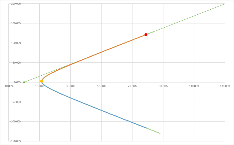
The Unconstrained Portfolio/ Free Problem provides no constraints on the weights of securities, and it is assumed that investors may use every technique that exists to construct their portfolios (table 2-3, and figure 1).

Under the unconstrained scenario, the minimal variance portfolio has a return of 2.57% and a standard deviation of 11.48%, with a Sharpe ratio of 0.224. The optimal portfolio, a portfolio with the maximum Sharpe ratio, has a return of 121.12 and % standard deviation of 78.78%, with a Sharpe ratio of 1.537.

3.2.  “Box” constraint |w_i| <= 1

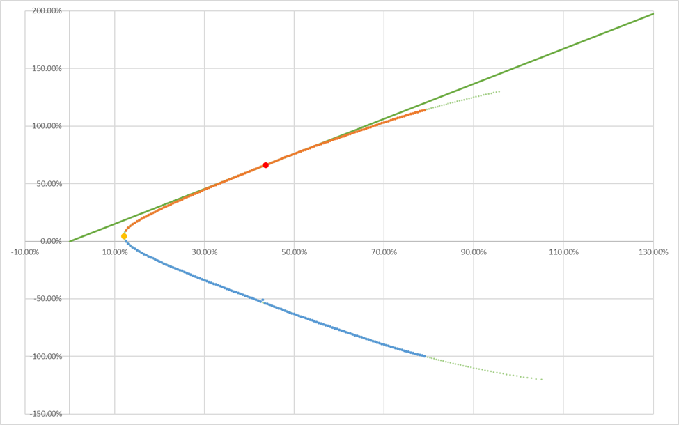
The “box” constraint used for comparison in this paper limits the weight investors may allocate to each of the securities within the portfolio. Particularly in this scenario, it is limited to  $$ -1\le w_i\le 1$$  or |wi| ≤ 1. Meaning that the absolute weight of any individual security may not surpass 100% of the portfolio.

The results is shown in table 4-5 and figure 2. Under the “box” constraint, where the absolute value of the weight of a single security must not exceed 1, the minimal variance portfolio had a return of 4.72%, a standard deviation of 12.03%, and a Sharpe ratio of 0.392. The optimal portfolio has a return of 66.23%, a standard deviation of 43.61%, and a Sharpe ratio of 1.519.

3.3.  Comparison

3.3.1.  Minimal variance

It is observed that the weights for the minimal variance portfolios in both scenarios are well diversified, with no single security’s weight exceeding 25%, except for the S&P index. This result is consistent with the assumptions of the Index Model, where diversification can eliminate firm-specific risk; thus, the minimal variance portfolio should be more diversified [10]. The major difference is that the unconstrained scenario allocated 181.87% of the weight to the S&P index, whereas the “box” constraint limited the weight of the S&P index to 100%.

It is also worth noting that under the unconstrained scenario, the index model was able to construct a portfolio with a standard deviation of 11.48%, whereas under the “box” constraint, the minimal variance portfolio has a standard deviation of 12.03%. This complies with the research hypothesis that an unconstrained scenario enables more combinations, and therefore, its efficient frontier contains a greater area than the “box” constraint. The “box” constraint’s minimum variance portfolio has a higher Sharpe ratio compared to the unconstrained scenario, making it more efficient.

3.3.2.  Optimal portfolio

The effect of the “Box” Constraint on the Index Model is more conspicuous when observing the optimal portfolios of the two scenarios. The unconstrained scenario has more concentrated weights with multiple securities’ absolute weights above 100%, meaning that more weight has been allocated to the few stocks that have extraordinary returns. In contrast, the absolute weights allocated to each security in the “box” constraint never exceed 100%. To illustrate the difference, five of the securities with the greatest absolute weight are listed in Table 6.

It is worth noting that LIN, AAPL, and UNP are stocks with the highest return-to-standard-deviation ratios within their own industry. Each was respectively 0.7623, 1.0445, and 0.7296. This combination guarantees a high return while pertaining diversification into various industries, providing a valid reason for the Index Model to prefer a more concentrated weight in these securities.

However, ACN’s high concentration was due to another factor, as it had a return-to-standard-deviation ratio of 0.6913, only the third-highest in the Technology sector. A potential explanation for why ACN was among the most concentrated stocks is due to its second-highest correlation of 71.3% with the S&P index, slightly lower than EMR’s 76.04%. A higher concentration of ACN would be able to hedge against the large negative weight allocated to the index. Though why ACN was preferred over EMR is not completely clear, this can be partly explained by its higher return-to-standard-deviation ratio compared to EMR’s 0.4138, making it a more attractive choice when searching for a combination with the highest Sharpe Ratio.

A cross-comparison reveals that the optimal portfolio for the “box” constraint generates a slightly lower Sharpe ratio than the unconstrained scenario. Meaning that it eliminated potential combinations with higher concentration and also higher risk-adjusted returns. Such an observation is consistent with the research hypothesis. Although the Sharpe ratio remained close in both scenarios, the return and standard deviation of the unconstrained scenario were around 1.8 times the values of the “box” constraint. This implies the Index Model under the unconstrained scenario tends to construct high-risk and high-return portfolios. This phenomenon is because the unconstrained scenario allows unlimited short selling and thus, theoretically, is capable of constructing portfolios with returns as high as desired at the cost of increasingly high risk [11].

The “box” constraint’s less concentrated portfolio limits the firm-specific risk a portfolio may take through diversification. The standard deviation,  $$ \sigma \left(e_p\right)$$ , of the unconstrained scenario and “box” constraint scenarios are respectively 71.68% and 38.19%. The risk and return trade-off is hence also limited, and the “box” constraint eliminates some portfolios with high risk and return. It is worth noting that under the box constraint, the Index model is unable to generate a portfolio with a return less than -120%.

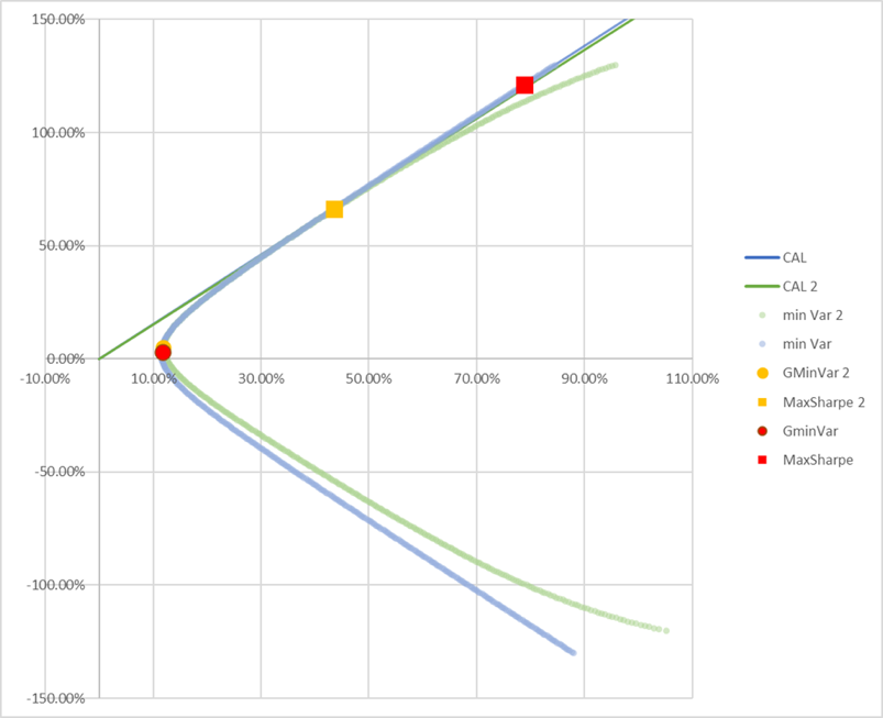
The graphical demonstration of the observations mentioned earlier also reveals that the unconstrained scenario has a slightly steeper CAL, which is consistent with the higher Max Sharpe ratio (figure 3). The graph of unconstrained efficient frontiers is almost linear toward higher standard deviations; in contrast, the efficient frontier for the “box” constraint is parabolic. A result of restricting unlimited short selling mentioned earlier. As the hypothesis predicted, the unconstrained frontiers cover a greater area; however, the differences occur mostly on the inefficient frontier and portfolios with high standard deviations. Suggesting that the constraint effectively excludes portfolios that take on unnecessary risk and rely on excessive short-selling, which are impractical in reality. Rational investors will not take on portfolios that use excessive short selling.

4.  Conclusion

This study applied the Single Index Model to a portfolio of the S&P 500 index and 21 stocks to analyze the impact of constraints on portfolio construction. The comparison between an unconstrained "free" scenario and a "box" constrained scenario yielded clear and theoretically consistent results.

The analysis is consistent with the hypothesis that the unconstrained efficient frontier dominates the constrained frontier, covering a greater area in the risk-return space. This is evidenced by the unconstrained model's ability to achieve a lower global minimum variance and a higher maximum Sharpe ratio, facilitated by its freedom to employ significant short selling to achieve any level of return required. In contrast, the box constraint limited concentration and leverage, resulting in a more diversified optimal portfolio with lower absolute risk and return.

While the unconstrained model is theoretically superior, its optimal portfolio requires extreme short positions and leverage that are often infeasible for real-world investors. The box constraint, though slightly less efficient, produced a more realistic and implementable set of portfolios by eliminating these impractical, high-risk combinations. This effectively demonstrates a key trade-off in portfolio management: constraints necessarily reduce theoretical efficiency but simultaneously enhance practical applicability by enforcing diversification and limiting exposure to excessive firm-specific risk.

Ultimately, this exercise successfully verifies fundamental portfolio theories and provides a practical supplement to textbook finance, illustrating how the Index Model behaves under realistic limitations and highlighting the critical balance between theoretical optimization and practical implementation.

References

[1]. Fama, E. F., & French, K. R. (2015). A five-factor asset pricing model. Journal of Financial Economics, 116(1), 1–22.
[2]. Chiah, M., Chai, D., & Zhong, A. (2015). A better model? an empirical investigation of the Fama-French five-factor model in Australia. SSRN Electronic Journal.
[3]. Fama, E. F., & French, K. R. (2018). Choosing factors. Journal of Financial Economics, 128(2), 234–252.
[4]. Ye, J., Wang, Y., & Raza, M. W. (2022). The Sharpe ratio’s upper bound of the portfolios in the presence of a benchmark: Application to the US financial market. Journal of Mathematical Finance, 12(03), 566–581.
[5]. Mistry, J., & Khatwani, R. A. (2023). Examining the superiority of the Sharpe single-index model of portfolio selection: A study of the Indian mid-cap sector. Humanities and Social Sciences Communications, 10(1).
[6]. Antypas, A., Koundouri, P., & Kourogenis, N. (2013). Aggregational Gaussianity and barely infinite variance in financial returns. Journal of Empirical Finance, 20, 102–108.
[7]. Sharpe, W. F. (1963). A simplified model for portfolio analysis. Management Science, 9(2), 277–293.
[8]. Abate, G., Bonafini, T., & Ferrari, P. (2022). Portfolio constraints: An empirical analysis. International Journal of Financial Studies, 10(1), 9.
[9]. Jorion, P. (2003). Portfolio optimization with tracking-error constraints. Financial Analysts Journal, 59(5), 70–82.
[10]. Napon, J. C. (2023). Brief Review on Asset Selection and portfolio construction: Diversification, risk and return. SSRN Electronic Journal.
[11]. Alemanni, B., Maggi, M., & Uberti, P. (2021). Unleveraged portfolios and Pure Allocation Return. Journal of Risk and Financial Management, 14(11), 550.
Cite this article
Yang,M. (2025). The Effect of Constraint on Portfolio Construction Using the Index Model. Advances in Economics, Management and Political Sciences,229,125-133.
Data availability
The datasets used and/or analyzed during the current study will be available from the authors upon reasonable request.
Disclaimer/Publisher's Note
The statements, opinions and data contained in all publications are solely those of the individual author(s) and contributor(s) and not of EWA Publishing and/or the editor(s). EWA Publishing and/or the editor(s) disclaim responsibility for any injury to people or property resulting from any ideas, methods, instructions or products referred to in the content.
About volume
Volume title: Proceedings of ICFTBA 2025 Symposium: Data-Driven Decision Making in Business and Economics
© 2024 by the author(s). Licensee EWA Publishing, Oxford, UK. This article is an open access article distributed under the terms and
conditions of the Creative Commons Attribution (CC BY) license. Authors who
publish this series agree to the following terms:
1. Authors retain copyright and grant the series right of first publication with the work simultaneously licensed under a Creative Commons
Attribution License that allows others to share the work with an acknowledgment of the work's authorship and initial publication in this
series.
2. Authors are able to enter into separate, additional contractual arrangements for the non-exclusive distribution of the series's published
version of the work (e.g., post it to an institutional repository or publish it in a book), with an acknowledgment of its initial
publication in this series.
3. Authors are permitted and encouraged to post their work online (e.g., in institutional repositories or on their website) prior to and
during the submission process, as it can lead to productive exchanges, as well as earlier and greater citation of published work (See
Open access policy for details).