1. Introduction

Against the backdrop of continuous deepening and innovation in the global financial system, market volatility has become a central focus for both academia and industry. In finance, volatility is used to reflect the degree and speed in which asset prices change over time, and it also represents the level of uncertainty and risk in expected returns. It is often quantified using the standard deviation or variance of logarithmic returns, which helps capture market expectations about future risk [1]. The volatility of financial markets is not only reflected in the fluctuation of short-term prices, but also in the macroeconomic environment due to investors' expectations, capital flow and policy transmission mechanism. In recent years, with the rise of high-frequency trading and the expansion of derivatives markets, volatility has exhibited increasingly complex and diverse characteristics. For instance, during periods of major policy adjustments, geopolitical conflicts, or unexpected public events, volatility tends to surge sharply, triggering risk-averse behavior among investors and amplifying systemic risks in capital markets. Therefore, studying the dynamic characteristics and measurement methods of financial market volatility can provide deeper empirical insights for theoretical research, as well as forward-looking risk warnings and decision-making references for investors and policymakers. The main purpose of this paper is to study the characteristics of financial market volatility and its measurement and forecasting methods in order to provide more understanding of market risk. In recent years, scholars have made significant progress in the study of financial market volatility. Numerous empirical studies emphasize the persistence and clustering effects of volatility, finding that volatility often remains high for extended periods and exhibits strong asymmetry—negative shocks tend to have a more pronounced impact on future volatility [2,3]. Meanwhile, the development of high-frequency data has facilitated the evolution of methods such as realized volatility and bipower variation, enabling researchers to capture intraday patterns and jump components of volatility with greater precision. On the other hand, rough volatility models have gained widespread attention in recent years. Researchers have found that such models better explain the fractal and long-memory properties of volatility and outperform traditional models in fitting market phenomena such as implied volatility smiles [4]. In addition, some studies have sought to combine volatility with macroeconomic variables and liquidity indicators to explore its underlying drivers and transmission mechanisms [5]. Overall, existing research has achieved substantial progress in modeling methods and data granularity, but certain limitations remain. First, most studies focus on single markets, with limited cross-market comparisons. Second, although high-frequency data can reveal finer structures of volatility, it still faces challenges such as noise and estimation bias. Third, there remains a gap between theoretical modeling and practical risk management applications. These limitations provide both the motivation and direction for this study.

This paper systematically analyzes the characteristics and measurement methods of financial market volatility. Firstly, it examines the major characteristics of volatility, including thick tail distribution, volatility aggregation, leverage effect, long memory and roughness, which provide a theoretical basis for understanding market dynamics; Then, the applicability and prediction performance of unconditional historical volatility, GARCH model, high frequency realized volatility and rough volatility model are compared. Finally, the study summarizes key findings, identifies current limitations, and outlines potential directions for future research. This paper aims to build a comprehensive analysis framework integrating theory and empirical analysis, and provide reference for academic research and risk management practice.

2. Characteristics of financial market volatility

2.1. Non-normality of return distributions

In traditional financial theory, it is often assumed that the returns of financial assets follow a normal distribution, meaning that most returns cluster around the mean, and extreme fluctuations occur with very low probability. However, in real markets, asset returns frequently exhibit a distribution that is “more peaked in the center and thicker at the tails”—that is, a higher kurtosis (leptokurtosis) and heavier tails. Empirically, this is typically reflected by: sample kurtosis significantly greater than 3, slow decay of the tails (right/left tail probabilities far exceeding those of the normal benchmark), and rejection of the normality hypothesis under tests such as Jarque–Bera. This implies that using normal approximations in risk measurement systematically underestimates the probability and magnitude of extreme events.

Recent studies have provided complementary evidence along three paths: cross-market robustness, high-frequency characterization, and distributional fitting optimization. Watorek et al. analyzed multi-market samples before, during, and after crises and the COVID-19 period, showing that return tails conform to power-law behavior (including the inverse cubic law), and during shock periods, tails become thicker with increased arrival rates of extreme events [6]. Liu et al. used one-minute high-frequency data from the Shanghai and Shenzhen indices, precisely measured the return distribution and found that the leptokurtic and heavy-tailed characteristics are robust in the Chinese market across different stages, regimes, and volatility states [7]. Pokharel et al. conducted large-sample empirical studies on Laplace and generalized Laplace families (asymmetric Laplace, skewed Laplace, Kumaraswamy-Laplace), showing that these distributions systematically capture higher kurtosis and heavier tails of returns, outperforming classical fat-tailed models such as the Variance-Gamma distribution across most indices. This suggests a feasible path of “replacing Gaussian assumptions with Laplace-family distributions” [8].

2.2. Volatility clustering

Under the idealized random walk hypothesis, the first-order autocorrelation of returns is usually close to zero. However, in real markets, periods of low volatility tend to be followed by low volatility, and periods of high volatility by high volatility, resulting in a time-clustered pattern known as volatility clustering. This can be seen empirically by the significantly and slowly decaying autocorrelations in the absolute returns (|rₜ|) and squared returns (rₜ²). The Ljung–Box tests applied to these series reject the null hypothesis of “no autocorrelation”, while the ARCH-LM tests reveal a significant autoregressive structure in the residual variances. In high-frequency contexts, realized volatility (RV) and its multi-scale decompositions (e.g., daily/weekly/monthly) also reveal the clustering of high and low volatility intervals. This implies that assuming independent and identically distributed variances—as in normal risk frameworks—systematically ignores state dependence and persistence, leading to biased estimates of margin requirements, VaR/ES levels, and hedge frequencies.

Zhao used data from 15 developed and emerging stock markets, separated intraday and overnight returns and found significant volatility clustering in both, with stronger persistence overnight. Clustering exists across multiple time scales, though cross-clustering between the two types is weak, implying that prediction models and risk assessment windows should distinguish between intraday and overnight behavior [9]. Kayani et al. divided samples into pre-pandemic and pandemic periods and detected volatility clustering, leverage effects, and leptokurtosis in multiple stock indices. Clustering was more persistent and pronounced during COVID-19, suggesting that high uncertainty phases produce systemic clustering in volatility, impacting risk management [10]. For Chinese markets, Wang applied GARCH-type models to the Shanghai and Shenzhen composite indices and found strong ARCH/GARCH persistence and predictive improvement, confirming that conditional heteroscedasticity and clustering are robust features in emerging markets and must be explicitly modeled [11].

From a methodological and practical perspective, GARCH(1,1) can serve as a baseline model to capture short-memory persistence. If multi-scale information or rolling forecasts are needed, the HAR-RV model (daily–weekly–monthly) can be used. For asymmetry or fat tails, EGARCH/GJR-GARCH models with heavy-tailed errors (Student-t/GED/Laplace) improve robustness in tail estimation. In risk management, higher margins, shorter hedging intervals, tighter risk limits, and state-dependent VaR/ES backtesting during high-clustering periods provide more realistic exposure assessments than static Gaussian frameworks.

2.3. Leverage effects and asymmetry

Among the stylized facts of volatility, the leverage effect and asymmetry describe the phenomenon that negative price shocks increase future conditional variance more than positive shocks of the same magnitude. Intuitively, price declines raise firms’ financial leverage and trigger risk aversion and deleveraging behaviors, amplifying subsequent uncertainty. Statistically, this appears as a significantly positive coefficient on negative shocks (e.g., the threshold term in GJR-GARCH or the sign term in EGARCH), resulting in a “news impact curve” with a steeper response to negative shocks.

Recent literature provides evidence from three perspectives. First, cross-market robustness: Large-sample analyses of developed markets show that, under univariate asymmetric GARCH frameworks, returns on the NASDAQ 100 index respond more strongly to negative shocks in conditional variance. The asymmetry terms in both EGARCH and GJR-GARCH models are statistically significant, confirming the leverage effect as a stable feature of volatility distributions [12]. Second, amplification during shock periods: Comparative studies of multiple stock indices before and during COVID-19 reveal that not only did overall volatility levels rise, but asymmetry also intensified—bad news in crisis conditions produced stronger amplifying effects on future volatility [10]. Third, evidence from the Chinese market: Cheng et al. examined asymmetric volatility spillovers across commodities and Chinese sectoral stocks. Using GJR-GARCH to capture market-specific asymmetry and a time-varying parameter VAR-DY framework to identify “bad/good volatility” linkages, they found systemic negative amplification and time-varying asymmetric spillovers in related Chinese sectors [13].

2.4. Long memory and roughness

Long memory refers to the autocorrelation phenomenon of volatility (whether measured by |rₜ|, rₜ², or log(RVₜ). Its attenuation rate is extremely slow, which means that the impact of market shock will last for a long time. Volatility roughness emphasizes the irregular and non-smooth nature of volatility paths over short horizons, typically characterized by a Hurst exponent  $$ \mathrm{H}<0.5$$ . Empirical studies typically estimate  $$ \mathrm{H}\approx 0.1$$  for log-realized volatility [14].

Bennedsen et al. proposed a continuous-time framework that can take in both short - term roughness and long - term mean reversion, providing parameter evidence across multiple markets that volatility exhibits a dual structure—rough at short horizons and persistent over longer horizons [15]. Cont and Das revisited the question of whether volatility is necessarily “rough” from a statistical perspective, proposing a nonparametric roughness estimation method and arguing that microstructure noise in high-frequency data can induce apparent roughness. Thus, distinguishing true roughness from measurement artifacts is crucial in empirical analysis [16]. Takaishi examined changes in Hurst exponents before and after the pandemic across markets (DAX, Nikkei, Shanghai, volatility indices, and cryptocurrencies). The results indicate that the roughness of volatility increments (H) remained broadly stable across stock markets, though return and absolute-return series showed market-specific differences, suggesting that roughness is relatively robust yet exhibits cross-market heterogeneity [17].

3. Measurement and forecasting methods of volatility

3.1. Baseline method: historical volatility

Historical volatility estimates the unconditional variance of returns within a fixed-length rolling window and is the most fundamental measure of volatility.

$$$ r_t=\mathit{ln}{P}_t-\mathit{ln}{P}_{t-1}$$$(1)

Where,  $$ r_t$$  denote the daily logarithmic return, and  $$ n$$  denote window length; then the rolling sample variance is given by equation (2).

$$$ \widehat{{\sigma }_t^2}\left(n\right)=\frac{1}{n-1}{\sum }_{i=0}^{n-1}{\left(r_{t-i}-\stackrel{-}{r_{t,n}}\right)}^2$$$(2)

$$$ \stackrel{-}{r_{t,n}}=\frac{1}{n}{\sum }_{i=0}^{n-1}{r}_{t-i}$$$(3)

In practice,  $$ \widehat{{\mathrm{\sigma }}_t^2}\left(n\right)$$  is often annualized using a scaling factor. To enhance sensitivity to new information, the exponentially weighted moving average (EWMA) method is also commonly adopted as an alternative. Historical volatility does not rely on any conditional variance structure, is simple to compute, and has high interpretability—making it a natural benchmark for comparison across different models.

From an informational standpoint, historical volatility offers three primary insights. First, relative volatility levels — under a uniform annualized scale, higher values of  $$ \widehat{{\mathrm{\sigma }}_t}\left(n\right)\mathrm{ }$$ indicate greater short-term uncertainty in prices. Second, regime or state shifts — when markets transition from normal to stressed states, volatility often exhibits stepwise jumps, followed by gradual declines when normality resumes. Third, persistence evidence: prolonged periods of high/low volatility appear as plateaus in the rolling series, and therefore motivate the usage of conditional variance models to model persistence.

It should be noted that historical volatility is an unconditional model that cannot capture the continuous and jump components presented in volatility, nor the jump responsiveness in conditional variance. These issues will be addressed by conditional heteroscedasticity models and high frequency estimation methods later. Based on daily series of CSI 300 Index from 2020 to 2024, this study computes 21-day and 63-day annualized historical volatilities. The 21-day window approximately corresponds to one trading month, reflecting short-term volatility changes and offering higher sensitivity to recent risks; the 63-day window corresponds roughly to one quarter, smoothing short-term noise while capturing mid-term volatility levels. Comparing two time scales helps examine volatility dynamics and the stability of market risk expectations.

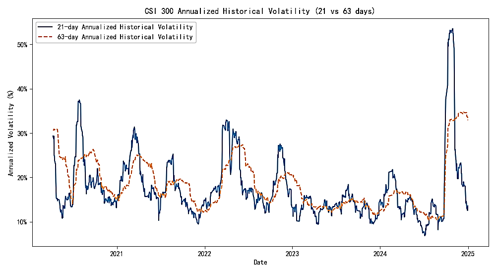
As shown in Figure 1, there are several volatility bursts caused by exogenous shocks in the sample period. The 21-day averege is responsive to state changes, while the 63-day averege is flatten and has a delay effect. High volatility periods will stay for several weeks or months before gradually subsiding. Volatility clustering and stickiness are displayed in Figure 1. When the 21-day volatility persistently exceeds and diverges from the 63-day level, it signals market “heating,” while convergence of the two suggests “cooling.”

3.2. The GARCH family of models

Compared with unconditional rolling estimates such as historical volatility, conditional heteroscedasticity models describe the dynamic evolution of volatility within a unified probabilistic framework. The central idea is that volatility is not constant—it varies over time and is driven jointly by past shocks and its own history.

In the most common GARCH(1,1) model, asset returns  $$ r_t$$  follow:

$$$ r_t=\mu +{\epsilon }_t$$$(4)

$$$ {\epsilon }_t={\sigma }_t{z}_t$$$(5)

where  $$ z_t$$  is an i.i.d. random variable with mean zero and variance one. The conditional variance evolves as:

$$$ {\mathrm{\sigma }}_t^2=\mathrm{\omega }+\mathrm{\alpha }\hspace{0.17em}{\mathrm{\epsilon }}_{t-1}^2+\mathrm{\beta }\hspace{0.17em}{\mathrm{\sigma }}_{t-1}^2,\mathrm{\omega }>0,\mathrm{ }\mathrm{\alpha },\mathrm{\beta }\ge 0,\mathrm{ }\mathrm{\alpha }+\mathrm{\beta }<1$$$(6)

In this framework, parameter  $$ \mathrm{\alpha }$$  captures the immediate impact of shocks on current volatility, while  $$ \beta $$  reflects the persistence or inertia of volatility. When  $$ \alpha +\beta $$  approaches one, volatility exhibits strong persistence, indicating a slow mean reversion and a long half-life of shocks.

To capture volatility clustering and generate comparable forward forecasts (useful for VaR/ES calculations and later model comparisons), this paper estimates a constant-mean GARCH(1,1) model based on daily logarithmic returns (in percentages) of the CSI 300 Index from 2020 to 2024. To better model fat tails and enhance robustness, the innovations follow a student-t distribution, and parameters are estimated via QMLE with robust covariance correction. The sample includes 1,210 trading days.

The estimation results of Table 1 show that  $$ \widehat{\mathrm{\alpha }}=0.0796$$  and  $$ \widehat{\mathrm{\beta }}=0.8777$$ , with their sum of 0.9572 corresponding to a volatility half-life of approximately 16 trading days, indicating significant persistence. The Student-t degrees of freedom are about 6.1, implying excess kurtosis above 5.8, much higher than the normal benchmark of 3, confirming heavy tails. The unconditional daily volatility is about 1.19%, with an annualized level of approximately 18.9%, consistent with historical volatility magnitudes. The mean term is close to zero, aligning with empirical properties of stock index returns. Overall, the GARCH(1,1) model effectively captures volatility clustering and fat tails within a concise framework, improving the depiction of extreme fluctuations.

However, there are several limitations. First, the model makes use of daily returns information only, hence it is not possible to take advantage of the rich information contained in high-frequency returns observed in trading. Second, the model is not able to identify jump component from continuous volatility, and therefore it may be biased during event-driven periods. Therefore, in more complex financial environments, the use of high-frequency data measures such as realized volatility (RV), bipower variation (BV) and the HAR-RV model is needed to improve both the granularity and the predictive ability of volatility models.

3.3. High-frequency data methods

Compared with methods relying solely on daily returns, high-frequency data approaches reconstruct volatility directly from micro-level price movements (minute-by-minute or tick-by-tick), providing a nonparametric and information-rich measure of realized volatility (RV).

If a trading day is divided into  $$ M$$  equal intervals, with high-frequency log-returns  $$ \{r_{t,i}{\}}_{i=1}^M$$ , realized volatility is defined as:

$$$ \text{R}{\text{V}}_{\text{t}}={\sum }_{i=1}^M{r}_{t,i}^2\mathrm{ }$$$(7)

Under a standard continuous semimartingale framework,  $$ \text{R}{\text{V}}_{\text{t}}$$  is an approximately unbiased estimator of the intraday volatility’s integrated variance. Its advantages include nonparametric robustness and high information content, allowing fine-grained observation of shock accumulation throughout the day.

However, RV is biased due to microstructure noise (e.g., bid-ask bounce, nonsynchronous trading). Excessive sampling frequency leads to an upward bias due to market frictions. Common corrections include sparse sampling, subsampling/smoothing, or pre-averaging to reduce the noise while keeping as much information of intraday volatility as possible.

To identify the contribution of jumps to total volatility, bipower variation (BV) provides a robust estimate of the continuous component:

$$$ \text{B}{\text{V}}_{\text{t}}={\mathrm{\mu }}_1^{-2{\sum }_{i=2}^M\left|r_{t,i}\right|\left|r_{t,i-1}\right|}$$$(8)

Where  $$ {\mathrm{\mu }}_1=\sqrt{2/\mathrm{\pi }}$$  . Under regularity conditions,  $$ \text{R}{\text{V}}_{\text{t}}-\text{B}{\text{V}}_{\text{t}}$$  approximates the contribution of jumps. This decomposition allows for empirical detection of jumps and analysis of event-driven volatility spikes. From a risk management perspective, when jumps dominate short-run risks, Gaussian-based conditional volatility frameworks are found to underestimate tail risk whereas the RV – BV approach offers direct support for state-dependent VaR/ES backtesting and stress scenario reconstruction.

At the forecasting level, the Heterogeneous Autoregressive Realized Volatility (HAR-RV) model explicitly integrates multi-scale memory to represent persistence and hierarchical structure in volatility. Its basic form is:

$$$ \text{R}{\text{V}}_{\text{t+1}}=c+{\mathrm{\beta }}_{\text{dR}{\text{V}}_{\text{t}}^{\left(\text{d}\right)}}+{\mathrm{\beta }}_{\text{wR}{\text{V}}_{\text{t}}^{\left(\text{w}\right)}}+{\mathrm{\beta }}_{\text{mR}{\text{V}}_{\text{t}}^{\left(\text{m}\right)}}+{\mathrm{\epsilon }}_{t+1}$$$(9)

Where  $$ \text{R}{\text{V}}_{\text{t}}^{\left(\text{d}\right)}=\text{R}{\text{V}}_{\text{t}}$$ ,  $$ \text{R}{\text{V}}_{\text{t}}^{\left(\text{w}\right)}$$  and  $$ \text{R}{\text{V}}_{\text{t}}^{\left(\text{m}\right)}$$  denote weekly and monthly averages, respectively. Unlike the single-lag GARCH model, the HAR-RV model employs a structured "daily-weekly-monthly" memory kernel to simulate the hierarchical inertia formed by investors and traders operating at different decision frequencies. It generally delivers robust performance in short-term (1–5 days) variance forecasting. Furthermore, researchers often integrate jump/continuous components within the HAR framework—for instance, using  $$ {\mathrm{B}\mathrm{V}}_t$$  and  $$ {\mathrm{R}\mathrm{V}}_t-{\mathrm{B}\mathrm{V}}_t$$  as explanatory variables—or incorporate additional information such as implied volatility, in order to capture forward-looking signals from the options market.

3.4. Frontier models: rough volatility

Traditional GARCH-type models effectively capture volatility clustering and asymmetry (through EGARCH or GJR-GARCH) in low-frequency data (daily or weekly), but the implied volatility paths are relatively smooth and fail to explain the short-term roughness widely observed in empirical data.

Recent literature shows that financial asset volatility (or its logarithm) exhibits fractal roughness with a Hurst exponent  $$ H<0.5$$ —that is, less smooth than Brownian motion ( $$ H=0.5$$ )—with correlations of increments decaying slowly with scale. Rough volatility models integrate short-term roughness and long-term mean reversion within a continuous-time stochastic process, providing unified explanations for both short-horizon dynamics and the shape of implied volatility smiles and skews.

Typical formulations include the RFSV and rBergomi models. The RFSV model assumes the log-volatility  $$ \log {\mathrm{\sigma }}_t=X_t$$  that  $$ X_t$$  process satisfies:

$$$ d{X}_t=-\mathrm{\lambda }\hspace{0.17em}\left(X_t-\stackrel{-}{X}\right)\hspace{0.17em}dt+\mathrm{\eta }\hspace{0.17em}d{W}_t^H$$$(10)

Where  $$ W_t^H$$  is a fractional Brownian motion with Hurst exponent  $$ H$$ ,  $$ \mathrm{\lambda }>0$$  is the mean-reversion rate, and  $$ \mathrm{\eta }>0$$  controls roughness intensity. This setting makes  $$ X_t$$  show a rough irregularity of  $$ H<0.5$$  in the short term, and a mean regression and stability in the long term.

Correspondingly, the rBergomi model directly constructs the stochastic variance using a fractional kernel under the risk-neutral measure:

$$$ {\mathrm{\sigma }}_t^2={\mathrm{\xi }}_0\exp \mathrm{ }\left(2\mathrm{\nu }{\int }_0^t{\left(t-s\right)}^{H-1/2}\hspace{0.17em}d{B}_s-{\mathrm{\nu }}^2{t}^{2H}\right)$$$(11)

Here,  $$ \nu >0$$  controls the roughness amplitude,  $$ {\xi }_0>0$$  is the initial forward variance, and  $$ B_s$$  is a Brownian motion. With its concise kernel structure, the rBergomi model achieves outstanding performance in pricing short-term options and fitting the implied volatility surface, effectively explaining the slope and curvature of the smile.

Compared with existing approaches, rough volatility models offer several distinct advantages. Unlike the GARCH family, they incorporate short-term roughness ( $$ H<0.5$$ ) within their structural formulation while retaining long-term mean-reversion dynamics, thereby providing a unified representation of the dual features of “short-term roughness and long-term slow decay.” In contrast to high-frequency methods such as RV and HAR-RV, rough volatility models do not rely on ultra–high-frequency data; instead, through a continuous-time generative mechanism, they can reproduce both short-maturity implied volatility surfaces and short-term volatility paths with fewer parameters. Furthermore, due to its parsimonious structure and computational tractability, the rBergomi model demonstrates stronger explanatory power in derivative pricing than many traditional diffusion or jump–diffusion models.

3.5. Model forecasting and comparison

In order to evaluate the predictive ability of different models under a comparative framework, this study employs a rolling-window recursive estimation–out-of-sample forecasting approach. The estimation window is set to  $$ T=750$$  days, with forecast horizon being  $$ h\in \{\mathrm{1,5},22\}$$ . At each time point  $$ t\ge W$$ , each model estimates its parameters using the data set  $$ \{1,\dots ,t\}$$ and subsequently generates forecasts of conditional variance denoted by  $$ \widehat{{\sigma }_{t+h\mid t}^2}$$ . The realized variance proxy  $$ v_t$$ is constructed using the Rogers–Satchell (RS) range-based estimator, with the Parkinson (PK) and Garman–Klass (GK) estimators employed as robustness benchmarks. The evaluation employs three commonly used metrics: Quasi-Likelihood Loss (QLIKE), Mean Absolute Error (MAE), and Mean Squared Error (MSE). The Diebold–Mariano (DM) test is further applied to assess the statistical significance of differences in forecast losses. In addition, the one-step-ahead conditional variance forecasts  $$ \widehat{{\sigma }_{t+1\mid t}^2}$$  are mapped to VaR estimates under the Student-t distribution assumption, with coverage and independence backtests conducted using the Kupiec and Christoffersen procedures.

Within a unified rolling-forecast framework, this study compares the variance forecasting performance of four models—HistVar-21, GARCH(1,1)-t, HAR-RS, and RFSV-Lite—based on the CSI 300 Index.

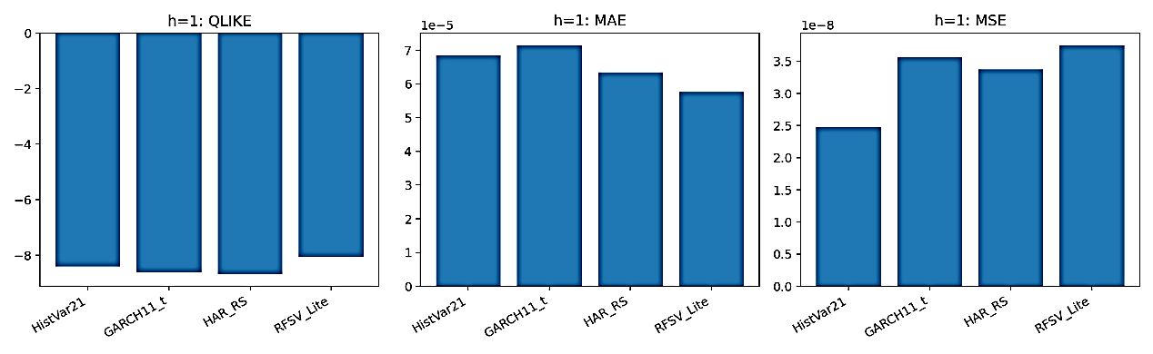
Regarding the point forecast accuracy metrics in Figure 2, the RFSV-Lite model significantly outperforms the others in QLIKE, which suggests that the rough volatility framework provides an improvement in modeling long-run volatility jumps. The HAR-RS model exhibits relatively stable performance on the MSE and MAE measures, comparable to that of the GARCH(1,1)-t model, and both models substantially outperform the unconditional HistVar-21 benchmark.

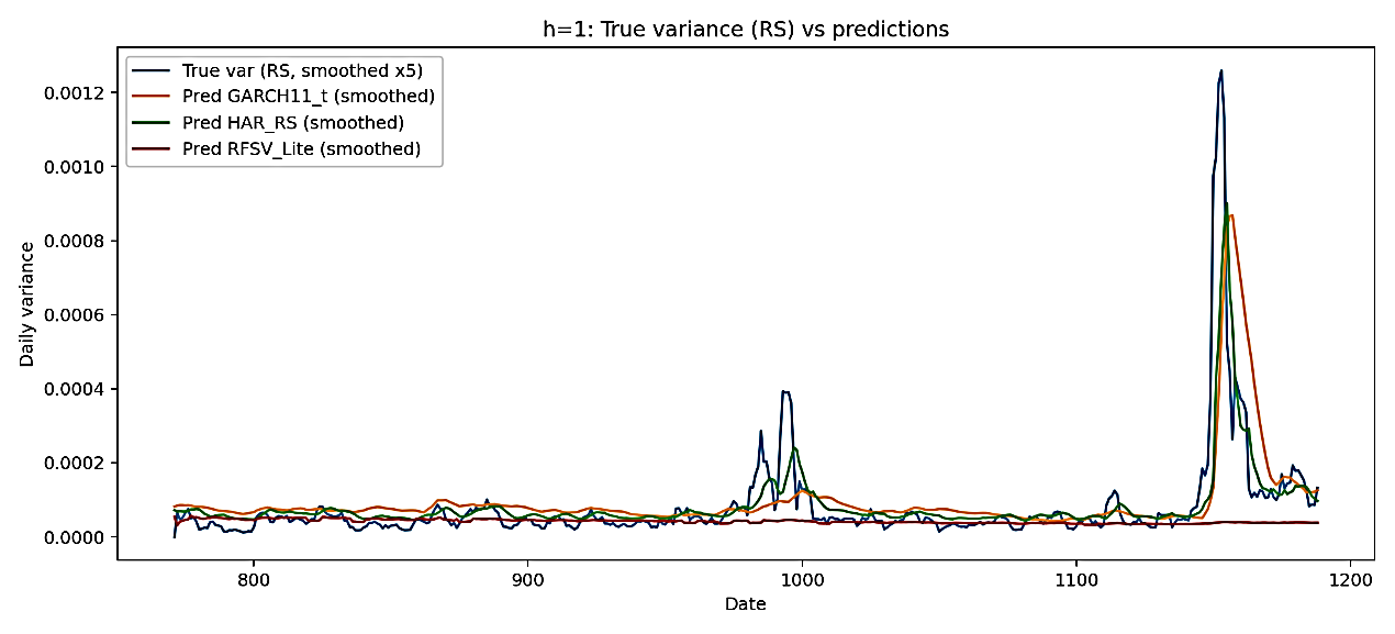
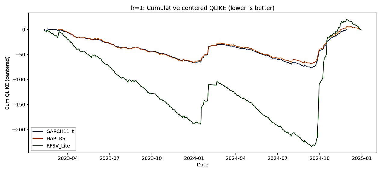
As illustrated in Figure 3, both the GARCH(1,1)-t and HAR-RS models effectively capture the “heating–cooling” dynamics of volatility, with their predicted paths closely aligning with the realized variance, particularly during the pronounced market fluctuations of 2023–2024. In contrast, the RFSV-Lite model produces comparatively smoother forecasts, exhibiting a tendency to underestimate volatility during high-turbulence periods while maintaining superior stability during calm market conditions. Furthermore, the cumulative QLIKE curves presented in Figure 4 indicate that RFSV-Lite consistently achieves the lowest cumulative forecast errors across most periods, confirming its advantage in overall predictive efficiency, though it displays jump-like deviations following extreme market events.

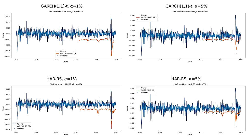
From a risk management perspective, the VaR backtesting results displayed in Figure 5 reveal that both conditional variance models can deliver good risk coverage in normal times, but the exceedances are quite clustered during extreme market stress periods (e.g., second half of 2024), which means that the tail risks are significantly underestimated by both models. Among them, the HAR-RS model shows an excessive number of violations at the 1% confidence level, reflecting a more pronounced issue of insufficient coverage, whereas the GARCH(1,1)-t model performs relatively more robustly but still demonstrates systematic bias under extreme volatility. Overall, the findings suggest that single-model approaches face inherent limitations in capturing extreme risk, implying that future research could explore ensemble modeling techniques or fat-tailed distributional adjustments.

In total, the four models exhibit different strengths in forecasting performance and risk management ability: RFSV-Lite is more accurate in the long run, while GARCH and HAR models are more sensitive to short-run changes. However, all models exhibit deficiencies in controlling tail risk, highlighting their potential complementarity and the value of integrated modeling approaches.

4. Conclusion

Based on the CSI 300 Index from 2020 to 2024 as the research sample, this study systematically analyzes the characteristics, measurement methods, and forecasting performance of financial market volatility. Research shows that the characteristics of financial market volatility have typical characteristics of heavy-tailed distribution, volatility clustering, leverage effects and long memory and roughness, reflecting the persistent and asymmetric dynamic evolution. Based on these findings, this study compares three categories of models: unconditional historical volatility, GARCH-type models that capture persistence and asymmetric reactions, and high-frequency realized volatility (RV) models that reflect multi-scale volatility transmission. The study also discusses the rough volatility framework, which uniformly characterizes short-term roughness and long-term mean reversion.

Empirical results show that GARCH(1,1)-t and HAR-RS perform relatively well in short-term forecasting, whereas RFSV-Lite achieves the best overall performance on the QLIKE metric, demonstrating a stronger capacity to capture long-term variance dynamics. However, VaR backtesting reveals that most models systematically underestimate tail risk during crisis periods, suggesting that single parametric models struggle to fully capture the characteristics of extreme returns.

The main limitations of this study are that the ultra-high frequency data are not widely used in continuous and jump component decomposition, and the traditional econometric models play a dominant role in forecasting. In the future, the research can further explore the high-frequency data, ensemble and regime switching model should be introduced, and the deep learning model based on LSTM or attention mechanism should be used to capture the non-linear and non-stationary characteristics. In addition, volatility forecasting can be extended to policy design – stress testing and macroprudential regulation, which has strong practical significance. Overall, this study reveals the complementary advantages of different models, providing valuable references for academic research and risk management practice.

References

[1]. Mieg, H. A. (2020). Volatility as a transmitter of systemic risk: Is there a structural risk in finance? Risk Analysis, 42(9), 1952–1964.
[2]. Ormos, M., & Timotity, D. (2024). Asymmetric volatility in asset prices: An explanation with mental framing. Heliyon, 10(3), e24978.
[3]. Trivedi, Jatin. (2022). Volatility Clustering Analysis: Evidence from Asian Stock Markets. The Empirical Economics Letters. 21. 99.
[4]. Bolko, A. E., Christensen, K., Pakkanen, M. S., & Veliyev, B. (2022). A GMM approach to estimate the roughness of stochastic volatility. arXiv.
[5]. Nguyen, L. T., Nguyen, M. T., & Nguyen, T. M. (2024). Asymmetric thresholds of macroeconomic volatility's impact on stock volatility in developing economies: A study in Vietnam. Journal of Economics and Development, 26(3), 224–235.
[6]. Wątorek, M., et al. (2021). Financial Return Distributions: Past, Present, and COVID-19.
[7]. Liu, P., et al. (2022). Precision Measurement of the Return Distribution Property Using High-Frequency Data from Chinese Stock Markets.
[8]. Pokharel, J. K., et al. (2024). Probability Distributions for Modeling Stock Market Returns: Evidence from Equity Indices.
[9]. Zhao, X. (2024). A multiscale analysis of intraday and overnight returns. Journal of Empirical Finance
[10]. Kayani, U. N., et al. (2024). Unleashing the pandemic volatility: A glimpse into the stock markets before and after COVID-19.
[11]. Wang, Y. (2022). Volatility analysis based on GARCH-type models. Economic Research-Ekonomska Istraživanja.
[12]. Aliyev, F., Ajayi, V., & Junttila, J. (2020). Modelling asymmetric market volatility with univariate GARCH models: Evidence from Nasdaq-100. Studies in Economics and Finance.
[13]. Cheng, S., Li, X., & Wu, X. (2023). Asymmetric volatility spillover among global oil, gold, and Chinese sector stocks. Resources Policy.
[14]. Gatheral, J., Jaisson, T., & Rosenbaum, M. (2018). Volatility is rough. Quantitative Finance, 18(6), 933–949.
[15]. Bennedsen, M., Lunde, A., & Pakkanen, M. (2022). Decoupling the short- and long-term behavior of stochastic volatility. Journal of Financial Econometrics
[16]. Cont, R., & Das, P. (2024). Rough volatility: fact or artefact? Sankhya B, 86(1), 191–223.
[17]. Takaishi, T. (2025). Impact of the COVID-19 pandemic on the financial market efficiency of price returns, absolute returns, and volatility increment: Evidence from stock and cryptocurrency markets. arXiv preprint arXiv: 2504.13051.
Cite this article
Wang,C. (2025). Analysis of Volatility Characteristics in Financial Markets: Evidence from the CSI 300 Index. Advances in Economics, Management and Political Sciences,239,52-64.
Data availability
The datasets used and/or analyzed during the current study will be available from the authors upon reasonable request.
Disclaimer/Publisher's Note
The statements, opinions and data contained in all publications are solely those of the individual author(s) and contributor(s) and not of EWA Publishing and/or the editor(s). EWA Publishing and/or the editor(s) disclaim responsibility for any injury to people or property resulting from any ideas, methods, instructions or products referred to in the content.
About volume
Volume title: Proceedings of ICFTBA 2025 Symposium: Data-Driven Decision Making in Business and Economics
© 2024 by the author(s). Licensee EWA Publishing, Oxford, UK. This article is an open access article distributed under the terms and
conditions of the Creative Commons Attribution (CC BY) license. Authors who
publish this series agree to the following terms:
1. Authors retain copyright and grant the series right of first publication with the work simultaneously licensed under a Creative Commons
Attribution License that allows others to share the work with an acknowledgment of the work's authorship and initial publication in this
series.
2. Authors are able to enter into separate, additional contractual arrangements for the non-exclusive distribution of the series's published
version of the work (e.g., post it to an institutional repository or publish it in a book), with an acknowledgment of its initial
publication in this series.
3. Authors are permitted and encouraged to post their work online (e.g., in institutional repositories or on their website) prior to and
during the submission process, as it can lead to productive exchanges, as well as earlier and greater citation of published work (See
Open access policy for details).