1. Introduction

The stock index is one of the most significant indicators of a nation's stock market performance. Almost all investors must analyse the trend of the stock index, which may indicate investor attitude regarding the state of the economy. The United States and China, hold market shares of 24% and 14% worldwide, respectively. The consistency of the stock market's development tendency in two nations with distinct economic systems over the past few years, under the influence of different policies and against the backdrop of diverse events, will have a direct impact on economists' assessment of economic globalization. At the same time, this problem's examination will help us appreciate the relationship between the two stock markets so that the potential of stock market crash caused by other country’s stock volatility could be prevented. S&P 500 and CSI 300, as the two most representative comprehensive stock indices in these two countries, will be useful in determining if the fluctuation of one country's stock market will affect other countries.

Various investigations have been launched on the Chinese and American stock markets in recent years. Using wavelet analysis, Gao and Ren have determined the affection of COVID-19 on the volatility of the Chinese and U.S. stock markets [1]. They believe that the COVID-19 has a substantial leverage effect on the U.S. and Chinese stock markets. Feng, Lucey, and Wang have explored the impact of the trade war between U.S. and China on the stock markets [2]. Using the VAR model to examine the SSE Composite Index and the S&P 500, the authors discover that the trade war has a beneficial effect on the U.S. stock market but a negative effect on the Chinese stock market. David, Broadstock, and George Filis analysed the oil price variation affection to the stock market [3]. Using the VAR model, they conclude that the U.S. stock market is more susceptible to swings in oil prices than the Chinese stock market. Amanjot SINGH and Parneet KAUR have identified the impact of the subprime mortgage crisis on the U.S., Indian, and Chinese stock markets [4]. Using the Tri-Variable Vector Autoregression approach, it was determined that the volatility of the U.S. stock market has an indirect effect on the volatility of the Chinese market via the Indian market. Caroline Geetha, Rosle Mohidin, Vivin Vincent Chandran, and Victoria Chong investigated the relationship between inflation and the stock market and discovered that the United States and Malaysia have a long-term equilibrium relationship between the inflation variables, whereas China has only a short-term equilibrium relationship [5]. Goh, Jiang, Tu, and Wang have examined if US economics can predict the Chinese stock market [6]. They conclude that the Chinese market is less predictable than the U.S. stock market using a basic predictive regression model. Farzad Farsio and Shokoofeh Fazel have conducted research on the relevance of predicting unemployment and the stock market [7]. Utilizing a discount cash flow model, they determined that using the unemployment rate to predict the stock market movement would be a mistake.

All of the aforementioned articles attempt to analyse single or numerous events that affect the two country’s stock market. However, few academics analyse the impact between those two countries stock markets directly. Hence, there is a greater impetus to perform extensive research on this area. Firstly, the stationarity of the model was examined using the data acquired from two stock indexes and plugged into the VAR model using the ADF and AR roots approach. Secondly, generating the influence time phase between two stock indices by utilising the impulse response function. Thirdly, quantify the influence between two stock indices using the variance decomposition method.

The remaining parts of this paper are constructed as follow. Part 2 depicts the data collection, part 3 introduce the method, part 4 reveal the results, part 5 shows the conclusion.

2. Data Collection

The data in this article are all collected from Investing (https://www.investing.com/). This paper selects the two representative stock indices from America and China. Those stock indices are S&P 500 (INDEXSP: .INX) and CSI 300 (SHA: 000300) for change percentage from 01/09/2021 to 01/09/2022. Since U.S. and Chinese stocks open times are different, then the data should be adjust and let the date match up. The change rate summarized in one chart is shown below in Table 1.

Table 1: Stock indices comparison statistic.

According to the table above, compare between the two stock indices, S&P 500 has the higher average return, the higher variance of return and the lower minimum rate of return. Vice versa, CSI 300 has the better Median return rate and higher maximum return rate. However, apart from the maximum data in the table, almost all other data are the same. That is a pretty good situation when continuing the study on the VAR model.

3. Methods

To start with, the Vector auto-regression (VAR) model is a stochastic process [8] model that is used to describe the relationship between variables when variation occurs. It is one of the most important model used in economics and natural sciences. By allowing multivariate time series, VAR models could generate stable single-variable auto-regressive model [9].

The VAR model with 2 variables are normally shown by 2 equations. The two equations are shown below,

\( {Y_{1,t}}= {C_{1}}+{α_{11}}{Y_{1,t-1}}+……+{α_{n1}}{Y_{1,t-n}}+{β_{11}}{Y_{2,t-1}}+……+{β_{n1}}{Y_{2,t-n}}+{ϵ_{1,t}} \) (1)

\( {Y_{2,t}}= {C_{2}}+{α_{12}}{Y_{1,t-1}}+……+{α_{n2}}{Y_{1,t-n}}+{β_{12}}{Y_{2,t-1}}+……+{β_{n2}}{Y_{2,t-n}}+{ϵ_{2,t}} \) (2)

In those above equations, \( {C_{1}} \) and \( {C_{2}} \) are the intercept which is the constant value. Combining \( {C_{1}} \) and \( {C_{2}} \) , could provide a 2×1 constant vector. \( {ϵ_{1,t}} \) and \( {ϵ_{2,t}} \) are the error value. Combining \( {ϵ_{1,t}} \) and \( {ϵ_{2,t}} \) could provide a 2×1 error vector. In the equation, from \( {α_{11}} \) to \( {α_{n1}} \) be the coefficients of the \( {Y_{1}} \) lags up to order n, where order n denotes that up to p \( {Y_{1}} \) lags are employed as predictors. Variables \( {Y_{1,t-1}} \) to \( {Y_{1,t-n}} \) describe the value \( {Y_{1}} \) from period t-n to t-1. Similarly, from \( {β_{11}} \) to \( {β_{n1}} \) be the coefficients of the \( {Y_{2}} \) lags up to order n, where order n denotes that up to p \( {Y_{2}} \) lags are employed as predictors. Variables \( {Y_{2,t-1}} \) to \( {Y_{2,t-n}} \) describe the value \( {Y_{2}} \) from period t-n to t-1. \( {α_{11}} \) to \( {α_{n1}} \) , \( {β_{11}} \) to \( {β_{n1}} \) , \( {α_{12}} \) to \( {α_{n2}} \) and \( {β_{12}} \) to \( {β_{n2}} \) will form an 1×n order matrix. In light of the aforementioned information, it is possible to deduce that the VAR model describes that A is affected by the prior periods of A's affectation and B's affection. Likewise, \( {Y_{2,t}} \) is also constructed with the same structure.

4. Results

The first section of the outcome describes the Augmented Dickey-Fuller test (ADF). The second section of the results pertains to the stability test, which is depicted by the graph of AR roots. In the third section of the results, the impulse response function and its accompanying images are discussed. In the concluding portion of the results section, the variance decomposition analysis is discussed.

4.1. ADF Tests

The initial step of our experiment is to find the number of difference required to make the series stationary. The ADF test is one of the most convenient and frequently performed test methods for testing stationary; therefore, the ADF test has been chosen to test the stationary. The ADF test is basically a statistical significant test. Normally the null hypothesis will be: series has a unit root. However, according to the result chart of CSI 300 shown below in Table 2. It indicates that the null hypothesis cannot be accepted. Therefore, the test of CSI 300 is stationary (See Table 2).

Table 2: ADF test for CSI 300.

Similarly, the test of S&P 500 is also stationary (See Table 3).

Table 3: ADF test for S&P 500.

4.2. Stability Test of VAR

It is required to assess the model's stability in order to produce a credible model estimate.When a model is stable, any variable sensitive to an external force can, as time passes, become less affected by the force until the system finds a new equilibrium. Nevertheless, if the model's stability is insufficient, the model will become meaningless as time passes. Hence, it worth to test the stability more carefully.

Initially, determining the optimal lag order in the criterion. The lag number has been set to 8 to determine the optimal lag sequence. The findings are shown in the table below in Table 4.

Table 4: Lag order test.

The lag order selection above is based on sequential modified LR test statistic, Final prediction error, Akaike information criterion, Schwarz information criterion and Hannan-Quinn information criterion. Due to the fact that lag order 1 has the greatest number of indicators. The lag order would then be set to 1.

According to the lag order 1 from above, the VAR estimation could be generated as below.

Table 5: VAR estimation.

Consequently, the AR root graph has been formed due to the data produced above. All the numbers in this graph are confirmed to be less than one, and all the points are contained within the unit circle. Therefore, the model under construction is stable (See Figure 1).

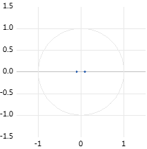
Figure 1: AR root graph.

4.3. Impulse Response Function

Based on the results demonstrated in the previous two sections, it is reasonable to believe that the data system is stationary. In the stationary system, the variation of the system to the input will be tracked by the impulse response function and being record as the following graphs. Figure 2 and Figure 3 depict the VAR model’s impulse response diagram for the two stock indices rate of change. The horizontal axis displays the respective response time periods, while the vertical axis depicts the variable's response to a standard deviation shock of one unit. The area within the two red dotted lines are the 95% CI and the black line in the middle is the impulse response locus.

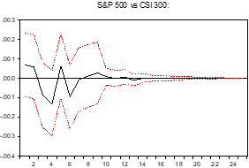
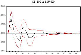
Figure 2 shows the response of S&P 500 to CSI 300 index. In the first time period, the initial impact of one standard deviation on the rate of change of CSI 300 for the S&P 500 is around 0.0006. Then, the positive and negative influences are continue alternating. The most negative impact appears in the 4-th period which roughly reaches -0.0013. As the lag time period increases, the figure shows that the impulse response locus will eventually trend to 0. The impact from S&P 500 to CSI 300 will finally disappear approximately in the 14-th time period. According to the above graphic, it is possible to conclude that the influence of S&P 500 change rate fluctuations on CSI 300 is complex, involving both positive and negative effects.

The impact of CSI 300 on the S&P 500 could potentially be analysed from a different angle. Figure 3 shows the response of CSI 300 to S&P 500 index. In the first time period, the initial impact of one standard deviation on the rate of change of S&P 500 for the CSI 300 is hardly any. Then, start from the second time period the impact start to appear. The most positive impact appears in the second period which roughly reaches 0.0032 and the most negative impact appears in the 5-th time period which roughly reaches -0.0019. After that, the positive and negative influences are continue alternating. As the lag time period lengthens, it becomes evident that the impulse response location will eventually tend toward zero. The CSI 300’s influence on the S&P 500 will cease to exist around the 10-th time period. According to the two charts produced above, the conclusion could be reached is that: both CSI 300 and S&P 500 have a high capacity for self-adjustment.

4.4. VAR Variance Decomposition Analysis

There is a traditional statistical technique in multivariate analysis for revealing structures that simplify a large number of variables which is named variance decomposition [10]. Variance decomposition will generate the contribution of impact of all endogenous variables in the data set from the MSE of all the endogenous variables. In order to pinpoint the time period more precisely, it would be beneficial to analyse the stock index's rate of change in greater detail. In the variance decomposition table, it has 4 columns. The first column represents the lag time period, and being fixed to 30 periods. The column S.E. represents the variable's forecast error for each forecast horizon. The last two columns are the impact of all endogenous variables in the data set on the basis of their origin.

The Table 5 is the variance decomposition table of S&P 500.The table reveals that the affectation of CSI 300 to S&P 500 has stabilised at approximately 10.993% over time. The fluctuation between affectations becomes stable at the tenth period according to Table 5, which corresponds to the graph in the previous part.

The Table 6 is the variance decomposition table of CSI 300. The table reveals that the affectation of S&P 500 to CSI 300 has stabilised at approximately 2.77% over time. The fluctuation between affectations becomes stable at the fourteenth period according to Table 5, which is consistent with the graph in Section 5.3.

5. Conclusion

Recent information data indicate that the majority of study on the VAR model focuses on certain disciplines or industries. However, few academics analyse the correlation between the stock index change rates of two countries. This research examines the extent to which the S&P 500 and CSI 300 affect each other and themselves. By using the ADF test and AR root graph, the system's stability and stationary have been verified. Impulse Response function and variance decomposition function has analysed the affectation period. This essay could help the investors to analysis one stock and make better decision based on the other stock index. At the same time, it could help economist and politician to prevent the potential stock market crash caused by another country’s stock volatility.

Although the stock index change rate of the 2 investigated stock indices seems similar, some potential problems exist. The top three industries with the most significant weight in the CSI 300 are metals and non-metals (15%), finance and insurance (10.94%), and machinery and equipment (10.74%). The top three industries with the most significant weight in the S&P 500 are information technology (27.3%), health care (14.1%), and consumer discretionary (11.4%). Those data are collected from https://business.sohu.com/. The above data shows a vast difference between the index structures. That means the result and conclusion proven previously might be temporary. As the stock index structure varies, the result might also vary in the future.

References

[1]. Gao, X., Ren, Y., Umar, M.: To what extent does COVID-19 drive stock market volatility? A comparison between the US and China. Economic Research-Ekonomska Istraživanja 35(1), 1686-1706 (2022).
[2]. He, F., Lucey, B., Wang, Z.: Trade policy uncertainty and its impact on the stock market-evidence from China-US trade conflict. Finance Research Letters 40, 101753 (2021).
[3]. Broadstock, D. C., Filis, G.: Oil price shocks and stock market returns: New evidence from the United States and China. Journal of International Financial Markets, Institutions and Money 33, 417-433 (2014).
[4]. Singh, A., Parneet, K. A. U. R.: Stock market linkages: Evidence from the US, China and India during the subprime crisis. Timisoara Journal of Economics and Business 8(1), 137-162 (2015).
[5]. Geetha, C., Mohidin, R., Chandran, V. V., Chong, V.: The relationship between inflation and stock market: Evidence from Malaysia, United States and China. International journal of economics and management sciences 1(2), 1-16 (2011).
[6]. Goh, J. C., Jiang, F., Tu, J., Wang, Y.: Can US economic variables predict the Chinese stock market? Pacific-Basin Finance Journal 22, 69-87 (2013).
[7]. Farsio, F., Fazel, S.: The stock market/unemployment relationship in USA, China and Japan. International Journal of Economics and Finance 5(3), 24-29 (2013).
[8]. Nakajima, J.: Time-varying parameter VAR model with stochastic volatility: An overview of methodology and empirical applications.
[9]. Hatemi-J, A.: Multivariate tests for autocorrelation in the stable and unstable VAR models. Economic Modelling 21(4), 661-683 (2004).
[10]. Jian, Z., Kuang, M., Economics, S. O.: China Macroeconomic System Dynamic Conduct, Conduct Reliabilities and the Dynamic Mechanisms of Monetary Policy. Economic Research Journal (2015).
Cite this article
Zhao,Z. (2023). Research on Interaction Between Chinese and American Stock Index: A VAR Approach. Advances in Economics, Management and Political Sciences,16,1-8.
Data availability
The datasets used and/or analyzed during the current study will be available from the authors upon reasonable request.
Disclaimer/Publisher's Note
The statements, opinions and data contained in all publications are solely those of the individual author(s) and contributor(s) and not of EWA Publishing and/or the editor(s). EWA Publishing and/or the editor(s) disclaim responsibility for any injury to people or property resulting from any ideas, methods, instructions or products referred to in the content.
About volume
Volume title: Proceedings of the 2nd International Conference on Business and Policy Studies
© 2024 by the author(s). Licensee EWA Publishing, Oxford, UK. This article is an open access article distributed under the terms and
conditions of the Creative Commons Attribution (CC BY) license. Authors who
publish this series agree to the following terms:
1. Authors retain copyright and grant the series right of first publication with the work simultaneously licensed under a Creative Commons
Attribution License that allows others to share the work with an acknowledgment of the work's authorship and initial publication in this
series.
2. Authors are able to enter into separate, additional contractual arrangements for the non-exclusive distribution of the series's published
version of the work (e.g., post it to an institutional repository or publish it in a book), with an acknowledgment of its initial
publication in this series.
3. Authors are permitted and encouraged to post their work online (e.g., in institutional repositories or on their website) prior to and
during the submission process, as it can lead to productive exchanges, as well as earlier and greater citation of published work (See
Open access policy for details).