JEL Classification Numbers: C26, D63, F60, H11

1 Introduction

When economic globalization is sweeping the world, it is also encountering more opposition and criticism. Many opponents believe that globalization has deepened inequality, which has seriously affected social and economic instability. Therefore, exploring the effect of globalization on income inequality plays an important role in policy-making process. The relationship between them has been discussed in many empirical studies, while it is still unclear due to application of different economies, methods, data or other factors [1-5]. Based on this, analysis in this work is more applicable and can widely explain the phenomenon of multiple times and countries.

Firstly, datasets are relatively large and new which allow enough fluctuations in different countries and at different times. The large amount of data allows to take a five-year average and lag independent variables to reduce endogeneity. Secondly, the methodology is more consistent and robust. The existing literature is either based on fixed effect model, or taking changes [6], or using instrument variables [7]. In the work, different methods have been combined to get more consistent and convincing results. Thirdly, the work takes sufficient heterogeneity analyses. Most studies just discuss the difference between different regions and hardly investigate the reasons [6-7]. In this work, not only differences, but also causes have been investigated.

This work finds that trade globalization shows a significantly positive effect on income inequality within countries on average. And the result is robust after considering endogeneity and has passed a series of robustness checks. Compared with high income economies, the disequalizing impact of trade openness is diminishing and even turns to the opposite for lower income countries. Besides, trade globalization can increase income inequality for advanced economies, while the heterogeneous impact is more complicated in diverse emerging economies.

The rest of the paper is organized as follows. Section 2 introduces the background of the research, including theoretical, empirical analysis and descriptive evidence. Section 3 describes data sources and measurement. Section 4 illustrates identification method, that is fixed effect model and instrument variables method. Section 5 analyzes the empirical results in detail and embodies baseline results, instrument regression results and several robust checks. Section 6 shows the conclusion.

2 Background

2.1 Theoretical analysis

The Stolper-Samuelson theorem states that changes in the relative prices of goods, which may be resulted from trade, have a strong effect on returns of factors. In the absence of joint production, changes in the relative prices will raise the real returns of some factors and lower the real returns of others. The more specialised a factor is in export production, the more it will benefit from trade. Conversely, the more a factor is concentrated in import production, the more likely it is to lose from trade.

As a result, trade globalization affects importing and exporting country differently, for example, high income country exports more technology-intensive products and oppositely, emerging country will export more labor-intensive products and these two strategies will have different impacts on high-skilled and low-skilled workers in each country which will influence income inequality. This finding suggests that international trade, while raising the welfare level of the total country, does not benefit everyone, with some people seeing their incomes rise while others fall. International trade can have a substantial effect on income distribution in a country.

2.2 Empirical evidence

The Stolper-Samuelson theorem was supported by some empirical evidence. Lee [8] conducted a study of 14 European countries and found that globalization increased European income inequality. The Kuznets hypothesis is valid, mainly because FDI rewards skilled workers or creates high-income groups. Goldberg & Pavcnik [1] believe that income inequality has worsened with trade liberalization, and its influence channels include international trade, technological changes, etc. The special mechanisms of globalization affecting inequality vary by country, time. Bergh & Nilsson [6] find that there is an obvious positive correlation between international trade freedom and income inequality, and this correlation only occurs in middle- and high-income countries. Lang & Tavares [5] think income inequality within countries has been exacerbated by globalization, because in many countries the income gains brought by globalization have flown to the rich and may not affect the poor.

However, some papers believe that this theory is not in line with the reality. Zhou et al. [2] show that there is a negative correlation between the trade globalization and income inequality. Jaumotte [9] believes that trade globalization reduces inequality, while financial globalization exacerbates inequality. Lim & McNelis [3] find that globalization and inequality has a threshold effect. Some others are sceptical about the strong relationship. They believe that, many other factors such as policies, education level, technology are more important. For example, Basu & Stiglitz [4] find that the widening income gap between the rich and poor is mainly caused by the changes in public policies such as deregulation of the financial sector and so on.

2.3 Descriptive evidence

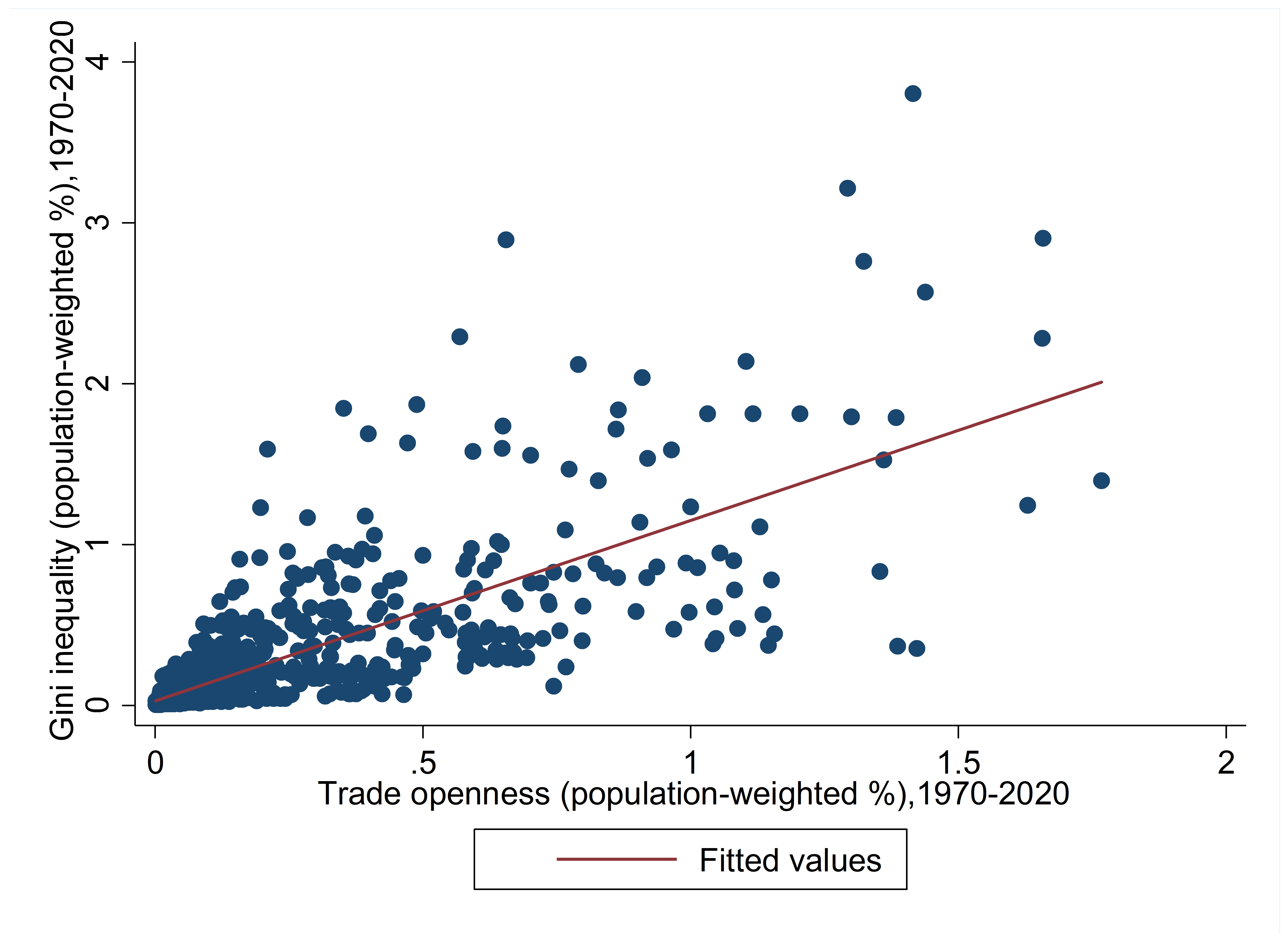
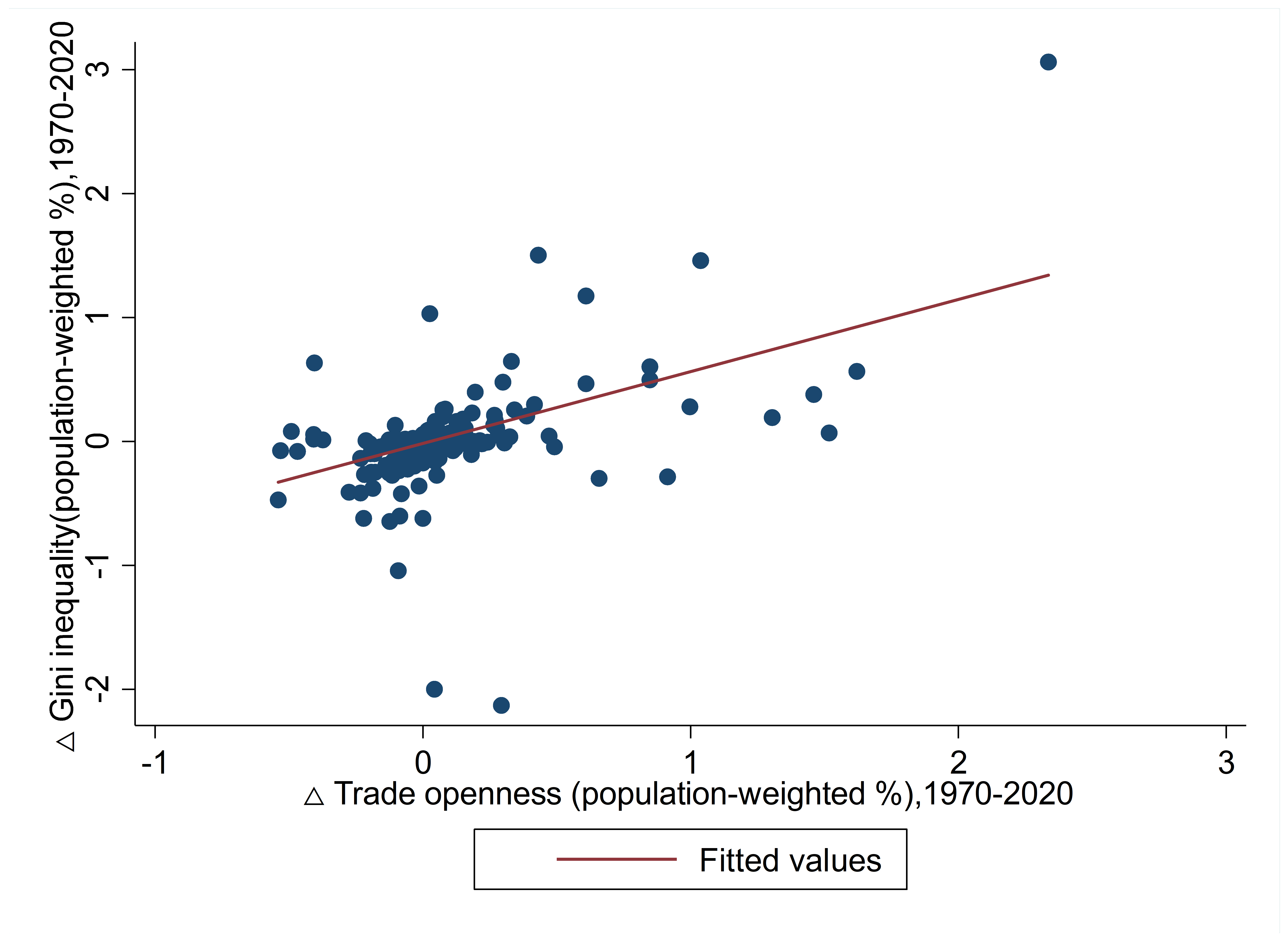
Fig. 1. Trade openness and gini inequality and changes in trade openness and gini inequality between the periods 1970–1975 and 2015–2020.

Note: Population weighted mean of the samples. Changes are defined as the next 5-year average values ( \( {period_{t+1}} \) ) minus the past 5-year averages ( \( {period_{t}} \) ).

Source: SWIID 9.0, World Bank (2020), Penn World Tables version 10, own calculations.

From Figure 1, trade globalization and Gini inequality always have positive relationship. Specifically, the correlation coefficient is 0.76 when measured in level, and the correlation coefficient is 0.50 when measured in change. However, causal relationship requires detailed empirical research.

3 Data Sources and Measurement

This work is based on an unbalanced panel data which consists of 166 countries from 1970 to 2018. In order to reduce the possible confused effect brought by outliers, missing values, measurement errors or short‐term movements, 5‐year averages of each variable are used. Data is from SWIID (Version 9.0) and PWT (version 10.0) [10]. The PWT is used for the measurement of trade globalization and control variables [11]. For comparison, this paper employs the KOF index of trade globalization from Swiss Federal Institute of Technology, Zurich [12].

Before empirical analysis, some transformations of data have been made. Such as, negative values of share of imports in GDP have been transferred into absolute value. 7 economies (including Singapore, Hong Kong, Belgium, Luxembourg, Malta, Djibouti and St. Kitts and Nevis) have been removed from the original data since they are outliers regarding trade openness and may bias the results.

The annual gini index of each country is used to measure domestic income inequality. Gini index of disposable income (post tax/transfer) and gini index of market income (pre tax/transfer) have the same trend over the sample period. To capture the effect of redistribution system within countries on income inequality, gini of disposable income is used as the dependent variable in empirical study. The sum of shares of merchandise exports and imports in output-side real GDP at current PPPs is used to measure trade openness. This key variable is closely related to the theoretical models the work referred and can help to have a thorough comprehension of the effect of trade globalization on income inequality. In the work, three important factors that affect income inequality are controlled. Technological change could adversely affect income distribution pattern by reducing the premium for lower-skill activities and rising the price for higher-skill activities [13]. Total factor productivity (TFP) is used to measure the pure technological progress in production. Economic growth and population changes are also likely to influence income distribution. The growth-inducing policies within countries also have effects on income distribution. GDP per capita is used to measure these effects. Higher education level can promote income equality, since it allows more people to be involved in high-skill jobs. Human capital index from Barro and Lee [14] and an assumed rate of return to education based on Mincer equation estimates is used to measure the role of education.

4 Identification Method

4.1 Fixed effect model

Based on panel data, this paper constructs the following fixed effect model and estimates this regression by ordinary least squares (OLS):

\( {Gini inequality_{i,t+1}}={β_{0}}+{β_{1}}×{Trade openness_{i,t}}+{β_{2}}×{X_{i,t}}+{α_{i}}+{γ_{t}}+{u_{i,t}}( SEQ "equation" \n \* MERGEFORMAT 1) \)

where \( i \) indexes each country, \( t \) indexes every 5-year period and all variables are averages of 5-year-period in a given country. \( {Gini inequality_{i,t+1}} \) describes the measure of income inequality of country \( i \) in period \( t+1 \) , to illustrate endogeneity problem, dependent variable is forwarded for one period in the regression. The independent variable \( {Trade openness_{i,t}} \) represents the trade openness of country \( i \) in period \( t \) . Additional control variables \( {X_{it}} \) include technology, economic development and human capital. \( {α_{i}} \) captures the country \( i \) fixed effects, which can eliminate country‐specific time‐invariant effects. \( {γ_{t}} \) describes the period \( t \) fixed effects, which can control for other period‐specific factors that may influence multiple countries at the same time. \( {u_{it}} \) is the error term. The paper estimates this panel fixed effect model with standard errors clustered at country level.

4.2 IV regression

There may be endogeneity in the baseline model caused by omitted variables and reverse causality. To address it, the instrumental variables approach is used.

Referring to Lang & Tavares, this paper uses the globalisation of the neighbouring countries as an instrumental variable [5]. Firstly, it satisfies relevance condition, due to geographical transmission, it is likely that a country’s trade globalization is highly correlated with its neighbor’s in the previous period. Then it also satisfies exogeneity condition, since it is impossible that the lagged value of trade globalization could affect income distribution through other channels except its own globalization score. So it is reasonable to use the neighbor’s trade openness as an instrumental variable.

IV is calculated using the following formula, where g is a measure of the degree of globalisation of a country's trade, and population-weighted distance is used to measure the distance between two countries [15].

\( {IV_{it-1}}=\frac{\sum _{j≠i}(\frac{1}{{distance_{ij}}}×{g_{jt-1}})}{\sum _{j≠i}\frac{1}{{distance_{ij}}}} ∀ j,i ∈I( SEQ "equation" \n \* MERGEFORMAT 2) \)

Regressions are done by two-stage least squares. The first stage regression is:

\( {g_{it-1}}=α{IV_{it-2}}+{X \prime _{it-1}}γ+{μ_{i}}+{ϑ_{t}}+{u_{it}}( SEQ "equation" \n \* MERGEFORMAT 3) \)

This equation is used to estimate the fitted values ĝ in the second stage regression. The regression equation for the second stage is:

\( {y_{it}}=β{g_{it-1}}+{X \prime _{it-1}}δ+{μ_{i}}+{ϑ_{t}}+{ε_{it}}( SEQ "equation" \n \* MERGEFORMAT 4) \)

Those variables are in different periods, IV is in the (t-2) period, trade globalization is in the (t-1) period and gini inequality is in the t period.

5 Empirical Results

5.1 Baseline results

Based on FE model, the results are presented in Table 1. In column 1, only the effects of country and period are considered, the regression yields a highly significant \( {β_{1}} \) of 0.0215 which suggests trade globalization plays a significantly positive effect on inequality. In column 2, whether there exists an inverted U-shaped relation is tested. In columns 3 to 5, control variables are added in turn, and all the results indicate that there is a significantly positive relationship.

Table 1. Baseline panel regressions of inequality on trade globalization

Note: Averages of 5-year periods. All independent variables are lagged for one period in the regression. Countries with extreme observations for trade openness have been excluded. Standard errors clustered at the country-level in parentheses, significance levels: * \( p \lt .10 \) , ** \( p \lt .05 \) , *** \( p \lt .01 \) . The same below.

5.2 Heterogeneity analysis

5.2.1 The role of income levels.

This paper further analyzes four subsamples classified by the income level of countries in Word Bank (WB) respectively: high income countries (44), upper middle income countries (45), lower middle income countries (34) and low income countries (26). The results are presented in Table 2. It can be seen that in columns 2 and 4, in high and upper middle income group, trade globalization has a significantly disequalizing effect. While in lower middle countries, column 6 shows that trade globalization has an equalizing impact at 1% confidence level. The results above are consistent with the S–S theorem. However, for low-income countries, trade openness does not affect income inequality, other factors such as technology and gdp per capita seem to be more important.

Table 2. Heterogeneity analysis of inequality and trade globalization (income levels in WIID)

5.2.2 The role of development levels.

Evidence shows that the heterogeneity is not significant if just spliting the world into advanced and developing economies. So the work looks into the more specific classification by IMF. In the World Economic Outlook (2021), advanced economies contains 3 economies, emerging market and developing economies contains 5. In this part, the heterogeneous impacts of trade openness across the 8 subgroups are analyzed and the causal factors behind are also explored. Results are shown in Table 3. The results from columns 1-3 shows that compared to emerging economies, trade openness has stronger disequalizing impact in advanced economies and it is most significant for the most advanced economies. The results for five subgroups of developing economies are shown in columns 4-8, they are diverse and have obvious regional heterogeneity. The interaction terms are significantly negative for Latin America and the Caribbean (-0.0568), but significantly positive for emerging and developing Europe. For other countries, the coefficients are insignificant. It should be noted that the heterogeneity cannot just be attributed to regional differences, other factors like technology, education, governance and policies may explain more. So this paper explores some causal factors in the following part.

Table 3. Heterogeneity analysis of inequality and trade globalization (development levels and regions, full sample)

(1) The role of technology. The baseline results are consistent with the hypothesis that technology progress will increase skill premium and widen income inequality. This work tests the heterogeneous impacts at different technology levels. The full sample is divided into five subsamples by tfp level from low to high (The regression results are omitted here, ask the author for it if interested). The results show that trade has equalizing impact in low technology level groups, but with the increase of technology, the equalizing impact is diminishing and changes to disequalizing impact. This may explain the disequalizing impact in European, as technology are higher.

(2)The role of education. The baseline results shows the increase in human capital can decrease gini. The work tests the heterogenous impacts at different education levels. Countries are ranked by human capital index and divided into five subsamples (The regression results are omitted here, ask the author for it if interested). The results show for the lowest education group, the disequalizing impact of trade is significant, with the improvement of education, the disequalizing impact is diminishing. This indicates that higher education level can alleviate the disequalizing impact of trade and can explain why the disequalizing impact of trade is lower in emerging Asia but higher in Africa. Since with rapid economic growth, emerging Asia has expanded investment in education, but education remains very low in many African regions.

(3)The role of export policies. Export-oriented policies can also affect income distribution. Large exports can lead to higher prices of goods and productivity in a sector, then increase income. The paper explores the impacts of export policies (The regression results are omitted here, ask the author for it if interested). By adding interaction terms between different exports and a dummy for advanced economies, it shows that both agricultural and manufactures exports have significant equalizing impacts in advanced economies. This is because agricultural and manufacturing jobs are both lower-paying jobs in these economies, larger exports in these sectors increase income for low-skill workers and thus reduce income inequality.

Further, this paper examines the impacts of exports in detail (The regression results are omitted here, ask the author for it if interested). The results shows that agricultural exports have significant equalizing impacts in some emerging countries with large agricultural exports share in the world or large agricultural exports share in its own exports, such as Brazil, Thailand. Also, it shows that manufactures exports can reduce gini in emerging and developing Asia, emerging and developing Europe and middle east and central Asia, but aggravates inequality in Sub-Saharan Africa. This is because in very underdeveloped African regions, manufacturing jobs are considered as higher-paying jobs the increase in manufactures exports increases income for high-paying workers and thus widens the income inequality.

Besides, this paper also explores the role of governance, redistribution policies and organizations. Due to limited space, the results are omitted. The results imply in countries with stronger governance in voice and accountability, political stability and absence of violence, government effectiveness and control of corruption, trade has equalizing impacts. As for redistribution policies, this paper uses government consumption share in GDP as an indicator of redistribution policies and finds that the effect of government consumption is ambiguous. Membership of some organization is probably not the causal factor, but country that meets the eligibility criteria has the economic, political and institutional structures that are important for reducing inequality. This paper tests these effects for two special organizations-EU and ASEAN-5, and finds the disequalizing impacts of trade is severer in European Union, but there is sizable equalizing impact in ASEAN-5. This can explain why trade has equalizing impacts in emerging Asia, but disequalizing impacts in emerging Europe.

5.3 IV results

IV regression results are shown in Table 4. In the first stage in column 2, IV has a significantly positive effect on trade openness and F tests also suggest IV is valid. In the second stage in column 1, the coefficient suggests that trade openness does have a positive effect on income inequality. However, Hausman test is insignificant which shows IV result is not significantly different from that of fixed effect model. This may because the main regression has solved lots of endogeneity problems and IV may not play an essential role. Therefore, the results are mainly based on fixed effect model.

Table 4. IV regressions of inequality and trade globalization

5.4 Robustness checks

The identification method mainly used is FE model and the above results suggest that it is credible. To ensure the consistency, this work takes robust checks in Table 5.

Firstly, this work considers whether there exists a long-term effect. Trade globalization is lagged by three periods to explore the impact of trade globalization 15 years ago on inequality now. From columns 1-2, trade globalization does have a long-term effect, and it is inverted U-shaped. When the level of trade globalization is relatively low, the increase in trade globalization increases inequality, but after a threshold (0.89), the increase can reduce inequality, but it only exists in the long run, and it is consistent with the main regression results. Secondly, the work discusses whether the deletion of outliers will bias the results. In the former analysis, some observations are deleted based on whether the ratio of import or export to GDP is greater than 1, which has excluded some abnormal values as well as some small countries. It may lead to problem of sample selection bias and underestimate the impact of trade globalization on inequality. Therefore, outliers are included to do a robust check. The results in columns 3-4 show that there still exists a significant positive effect, so the removal of outliers doesn't bias the results.Finally, considering the analysis based on level may ignore the specific time trends of each country, this work further analyzes the relationship based on changes, and the results in columns 5-6 show that trade globalization still has a significant positive effect on income inequality, which verifies that the main regression results are robust.

Table 5. Robustness checks of inequality and trade globalization

6 Discussion and Conclusion.

This paper uses data of 166 countries from 1970-2018 to investigate the impact of trade globalization on income inequality within countries. The results show that trade globalization has a significantly positive impact on income inequality on average. The result is robust after considering endogeneity and robustness checks. However, the impact may differ across country. Compared with high income countries, the disequalizing impact of trade openness is less pronounced for lower middle income group, which is consistent with the Stolper-Samuelson theorem. Using classification method from World Economic Outlook, the paper has a more systematic discussion on the heterogeneous impact and some other factors should be considered.

In detail, the improvement of education and governance can suppress the disequalizing impact of globalization since education can allow more to be engaged in high-skill jobs, and an effective government can regulate the implementation of policies related to income distribution. The improvement of technology aggravates the disequalizing impact since it can reduce the demand for lower-skill jobs and increase the premium for high-skilled activities. The role of export-oriented policy depends on the industry structure. Since agricultural and manufactural exports are both considered as low-skilled jobs in advanced economies, exports in those sectors have equalizing effect. As for emerging economies especially that agriculture accounting for a large percentage, agricultural exports exhibit a positive effect on income distribution. While in the underdeveloped economies of Sub-Saharan Africa where manufacturing is a higher-paying industry, increase in manufacturing exports deepen income inequality.

For all economies, although with the development of technology, it is natural to witness the deterioration in income distribution at specified period. However, it is still helpful to improve access of education and governance effectiveness to benefit the distribution of income. At the same time, flexible adjustment of export industrial structure is also a good way to improve the income distribution given that economy globalization and integration have been the trends of world development. It’s worth noting that, apart from the common factors used in inequality analysis, individual economy circumstances do vary. Therefore, policies need to be formulated for specific economy circumstances to ensure greater benefits from trade globalization.

Acknowledgement: These authors contributed equally to this work and should be considered co-first authors.

References

[1]. Goldberg, P. K., Pavcnik, N. (2007) Distributional effects of globalization in developing countries. Journal of Economic Literature, 45: 39–82.
[2]. Zhou, L., Biswas, B., Bowles, T., Saunders, P. J. (2011) Impact of Globalization on Income Distribution Inequality in 60 Countries. Global Economy Journal, 11: 1-18.
[3]. Lim, G. C., McNelis, P. D. (2016) Income growth and inequality: The threshold effects of trade and financial integration. Economic Modelling, 58: 403-412.
[4]. Basu, K., Stiglitz, J. E. (2016) Inequality and growth: patterns and policy. Palgrave Macmillan, New York.
[5]. Lang, V. F., Tavares, M. M. (2018) The Distribution of Gains from Globalization. IMF Working Paper, 18:1-1.
[6]. Bergh, A., Nilsson, T. (2010) Do liberalization and globalization increase income inequality? European Journal of Political Economy, 26: 488-505.
[7]. Dorn, F., Fuest, C., Potrafke, N. (2022) Trade openness and income inequality: new empirical evidence. Economic Inquiry, 60: 202–223.
[8]. Lee, J. E. (2006) Inequality and globalization in Europe. Journal of Policy Modeling, 28: 791-796.
[9]. Jaumotte, F., Lall, S. Papageorgiou, C. (2013) Rising Income Inequality: Technology or Trade and Financial Globalization. IMF Economic Review, 61: 271–309.
[10]. Solt, F. (2020) Measuring Income Inequality Across Countries and Over Time: The Standardized World Income Inequality Database. Social Science Quarterly, 101: 1183-1199.
[11]. Feenstra, R. C., Inklaar, R., Marcel, P. T. (2015) The next generation of the Penn World Table. American Economic Review, 105: 3150-3182.
[12]. Gygli, S., Haelg, H., Potrafke, H., Sturm, J. E. (2019) The KOF Globalisation Index – Revisited. Review of International Organizations, 14: 543-574.
[13]. Birdsall, N., Rodrik, D., Subramanian, A. (2005) How to help poor countries. Foreign Affairs, 84: 136–152.
[14]. Barro, R.J., Lee, J. W. (2012) A new data set of educational attainment in the world, 1950–2010. Journal of Development Economics, 104: 184-198.
[15]. Mayer, T., Zignago, S. (2011) Notes on CEPII’s distances measures: The GeoDist database. CEPII Working Paper, 25: 1-12.
Cite this article
Zhou,J.;Xue,J.;Liu,L. (2023). Trade Globalization and Inequality: Evidence Across Economies. Advances in Economics, Management and Political Sciences,3,122-132.
Data availability
The datasets used and/or analyzed during the current study will be available from the authors upon reasonable request.
Disclaimer/Publisher's Note
The statements, opinions and data contained in all publications are solely those of the individual author(s) and contributor(s) and not of EWA Publishing and/or the editor(s). EWA Publishing and/or the editor(s) disclaim responsibility for any injury to people or property resulting from any ideas, methods, instructions or products referred to in the content.
About volume
Volume title: Proceedings of the 6th International Conference on Economic Management and Green Development (ICEMGD 2022), Part Ⅰ
© 2024 by the author(s). Licensee EWA Publishing, Oxford, UK. This article is an open access article distributed under the terms and
conditions of the Creative Commons Attribution (CC BY) license. Authors who
publish this series agree to the following terms:
1. Authors retain copyright and grant the series right of first publication with the work simultaneously licensed under a Creative Commons
Attribution License that allows others to share the work with an acknowledgment of the work's authorship and initial publication in this
series.
2. Authors are able to enter into separate, additional contractual arrangements for the non-exclusive distribution of the series's published
version of the work (e.g., post it to an institutional repository or publish it in a book), with an acknowledgment of its initial
publication in this series.
3. Authors are permitted and encouraged to post their work online (e.g., in institutional repositories or on their website) prior to and
during the submission process, as it can lead to productive exchanges, as well as earlier and greater citation of published work (See
Open access policy for details).