1. Introduction

Equity market is where stock dealers and merchants who can buy and sell stock shares congregate. On stock exchanges, shares of numerous businesses are published. This improves the stock's liquidity, which attracts more purchasers [1]. Significant investments are made in the stock market by a large number of buyers. However, it carries risk due to the rapid rise and decline of asset prices.

Various methods to stock price prediction have been used. In the past, statistical approaches such as Exponential Smoothing and the Inexperienced Approach were utilized for forecasting stock prices [2]. Because statistical approaches are linear in character, they perform poorly in cases of sudden rises or falls in stock prices. For inventory information, which is unpredictable, erratic, arbitrary, and reliant on several technological variables, statistical methods have failed to be as dependable [3].

The main element of the typical financial sector forecast technique is time-series analysis. The traditional time-series analysis techniques encompass AR, ARMA and ARIMA [4-6].All of these techniques ignore other influential factors like the context data in favor of focusing mainly on the moment sequence itself. Aiming to determine the quantitative relationship between the earlier data and the later data, they specifically presume that they are independent and dependent variables, respectively. The stock market models and forecasts also handle a lot of data, which poses a significant challenge to the algorithm design. Traditional stock market predicting methods are inadequate as a result of these traits.

The rest of this essay is formatted as follows. Section 2 provides the model. The statistics used are described in Section 3. This article explains the graph topology and training labels in more detail. The experimental findings in Section 4 demonstrate the efficacy (and precision, in particular) of our suggestion. Finally, Section 4 also includes opinions.

2. Model

2.1. Linear Regression

Data with a numerical goal variable are predicted using linear regression. This study uses a mix of dependent and independent factors for making predictions. This part will use linear regression model when there is just a single dependent variable and an independent variable. It relies on the situation whether the regression pertains to a single variable or multiple ones [7].

In the figure 1, the blue rectangle is the residual and the red one is Normal Distribution line, it shows the residual difference between the forecasting result and the real worth.

According to R2, which refers to root mean square error, 0.7% of classifications generated via linear regression were erroneous but the remainder of the work was precise and error-free. Data on closing values from the month of December 2016 to November 2020 were used in this processing. For prediction, we only took date and closing rates into account [8].

2.2. Long Short-term Memory (LSTM)

A memory block's layout, which consists of gates and memory cells, is shown in Figure 2. At the time t, and,,and are the gateways, which, respectively, are known to as ignore, the output, and input gateways. andreact to the input and concealed state, respectively. The candidate input to be stored is, and an input gate later regulates the quantity of storage. Gateway includes input candidate, cellular state, and concealed state.

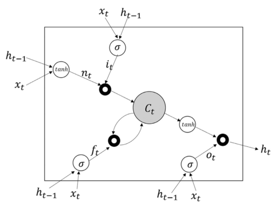
Figure 2: Structure of an LSTM memory block. (Source:https://www.sciencedirect.com/science/article/pii/S0957417418304342).

A and B are bias vectors and weight matrices. The sign for denotes element-by-element multiplication. The secret state is updated using tanh activation. In Fig. 2, sigmoid activation for gating is denoted by the symbol and is calculated via the sigmoid function.

The range [0, 1] encompasses the result. There is no information entry if the result number is zero. More details are allowed as the result figure rises, and information can be completely reflected if it reaches 1. Because of this selective information reflection, LSTMs can acquire longer temporal patterns [9].

2.3. Random Forest

Different machine learning apps could use decision trees. Nevertheless, trees gradually become very deep to acquire exceptionally erratic patterns tend to overstretch the exercise routines. Due to a minuscule amount of data disturbance, the tree may evolve completely differently. Decision trees' extremely low bias and large variance are the reason for this. RF circumvents this issue with numerous decision trees being trained on various areas within the characteristic spectrum at the expense of slightly greater bias. The complete training set is therefore invisible to any tree in the forest, according to this. Repetitively dividing the substance results in the creation of segments. By looking up a property at a particular node, the division is performed.

Gini impurity is utilized to evaluate the split's strength in every component. Below is the Gini impurity

P () is the population percentage with the label i. Shannon Entropy is a metric that could be applied to assess the peculiarity of a split. It assesses the degree of disarray in the information substance. Shannon Entropy is utilized in decision trees to gauge the volatility of data contained in a particular node of a tree's structure. (In this situation, It evaluates how mixed the populace in a node is). The following formula can be used to determine the volatility in a node N:

Bootstrap aggregation, also known as bagging, is at the core of every one of aggregate machine learning algorithms. This technique enhances both the precision and reliability of learning algorithms. It also lessens over-fitting and variance, which are prevalent issues when building decision trees, at the same time [10].

After the calculating in figure 3, the accuracy of the up and down prediction is 0.1515, which means the precision of Random Forest algorithm is slightly lower.

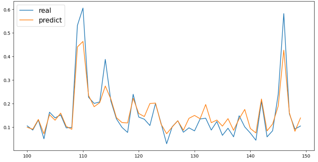
Figure 3: Test data of the AAPL stock price.

3. Data

3.1. Data Representation

This paper has demonstrated the sectional dataset of Apple stock. The reason whytaking up Apple stock is that it is a more consumer - friendly company, which has many end users worldwide. So, historical AAPL stock prices are taken for the period 2016 to 2021 from yahoo finance. And further, this dataset is divided into two parts. 4/5th portion of the data is used as training data and 1/5th portion as test.

To transform these CSV documents into tabular DataFrames that were categorized by date, the Python Scientific Computing package numpy was used in conjunction with a data analysis package. Each company is a perspective of the main DataFrame that has been filtered based on its ticker. This enabled quick entry to stocks that were intriguing as well as simple access to data categories.

Figure 4: The closing price of AAPL from 2016 to 2021.

In the figure 4. It is easy to see that Apple stock maintains a sustained growth trend over a five-year period, but fluctuates slightly during the year 2021, with an overall upward trend.

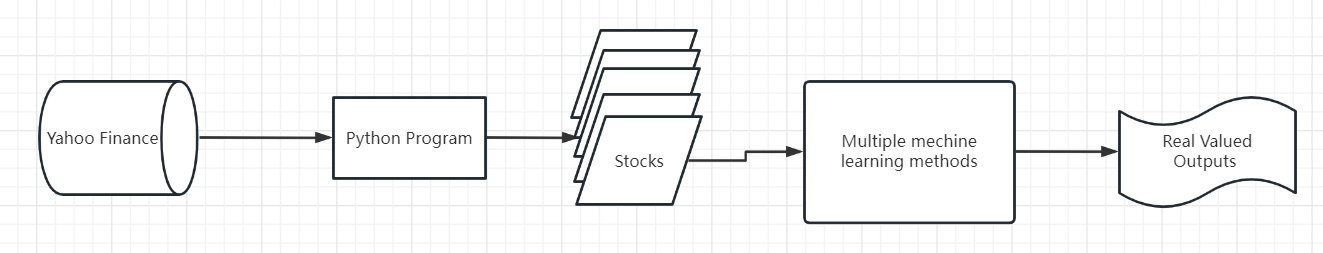
Figure 5: Data flow diagram illustrating the transformation of market data into forecast value vectors.

The flow chart in figure 5 illustrates how the program works and transform the initial data into the predicting ones.

3.2. Technical Index Data

3.2.1. Moving Average (MAVG)

In order to forecast the need for one or more future times, the Moving Average Approach employs a collection of current past criteria. It is one of the most widely used techniques for time series. When the previous demand weights are exactly the same for each time, the measure is referred to as a simple moving average; when the weights are distinct, the measure is referred to as a weighted moving average. A weighted moving average is used when the weights vary. The more recent the history of demand, the more weight is typically given in a weighted moving average, which means that the most recent information is given more weight, but all the weights sum up to one.

It is not difficult to see from the generated function image that compared with the actual value, the result obtained by moving average is generally lagged, which is equivalent to the transverse movement of the actual value.

3.2.2. Relative Strength Index (RSI)

Relative Strength Index (RSI): A momentum measure called the RSI can indicate when a security is oversold or overvalued. The RSI scale runs from 0 to 100; a company is deemed overbought when it exceeds 80 and oversold when it falls below 20. Other data categories, such as 70 and 30, or 90 and 10, are used by some researchers.

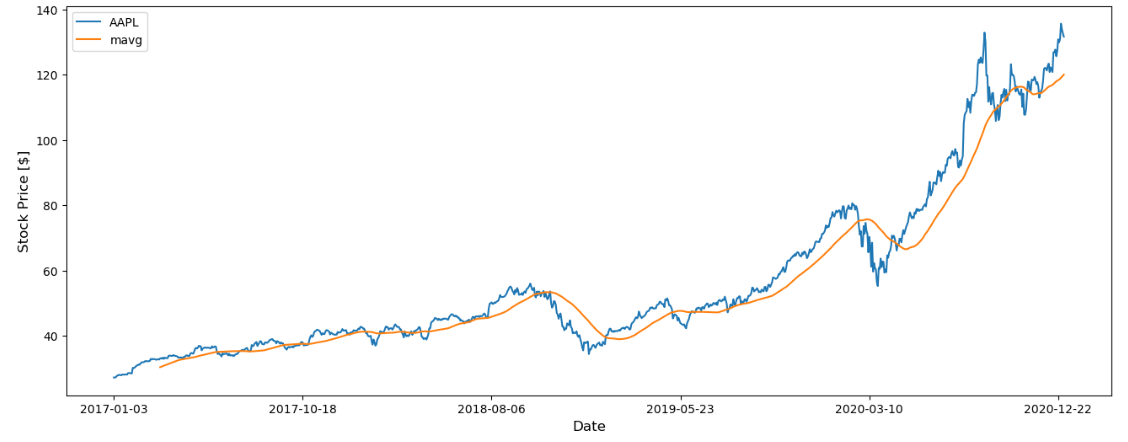
Figure 6: MAVG line compared to the AAPL close price line.

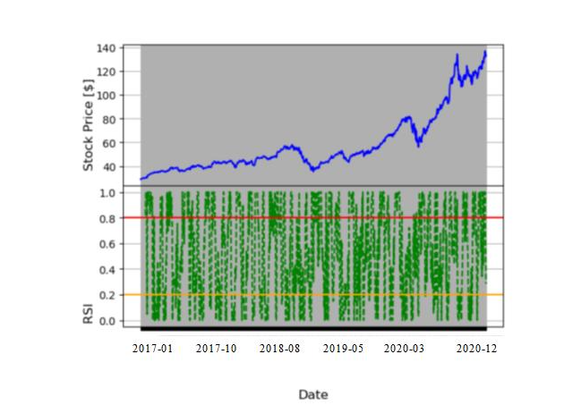
Figure 7:Technical index analysis chart based on relative strength index.

In this figure 7, above the red line is an overbought zone, increasing the chance of a market backstop, Below the yellow line is oversold area, market rebound opportunity increases. The RSI index should stay on the sidelines while halfway between the red and yellow lines.

3.2.3. MAE/MSE/RMSE

MAE: Mean Absolute Error, which can more accurately represent the real condition of predicted error.

MSE: Mean Square Error, The average of the squares of the inaccuracy at the locations where the forecasting information and the initial information are present is the statistical measure.

RMSE: Root Mean Square Error, Find the mean square error's square root.

Where, n is the sample number, is the predicted value and is the actual value.

4. Results

4.1. Calculating Returns

4.1.1. Linear Regression

Compared to polynomial regression approaches, linear regression was less susceptible to normalization methods. Some plausible results began to emerge at the beginning of the study, even with a few features that were not normalized, whereas this led to an excess in the polynomial regression models. Due to its streamlined model, linear regression also produced tenable results after normalization without the need for parameter tweaking, though the precision is lower than anticipated if we use the results to construct a portfolio.

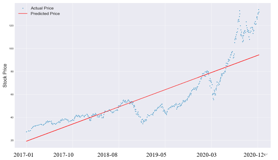
Figure 8: Forecasting the price of AAPL using linear regression.

4.1.2. Long Short-Term Memory (LSTM)

In this model, the LSTM layer is configured with 50 memory and output at each time step. Data with numerous input factors can be predicted using networks based on LSTM. A single time-dependent indicator determines the forecast in a univariate time series. Multivariate time series, in contrast to binary time series, can include several factors. These factors may be contingent on other values in addition to their historical value [11].

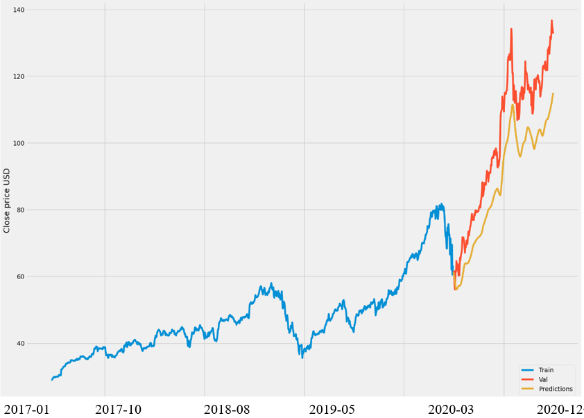
Figure 9: Predicting the price of the AAPL shares using Long-Short Term Memory.

This figure illuminates that that LSTM model can predict the future stock price more accurately, which is in good agreement with the actual price.

4.1.3. Random Forest and KNN

Random Forest: One of the groups learning algorithms is the Random Forest algorithm. It is a cumulative model that combines the outcomes of a series of decision trees to generate predictions.

KNN: A straightforward method called K-Nearest Neighbors can forecast number targets according to a similarity metric. KNN determines the average of the K closest neighbors' number objective.

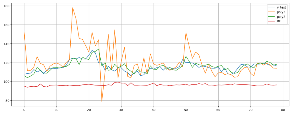
Figure 10: The comparison between Random forest and KNN model.

In figure 10, the red line depicts the Random forest model, and the light blue line indicates the KNN result, which is superior to RF.

4.2. Precision Returns

Both the MAE and MSE of LSTM are the smallest among the four machine learning models. LSTM networks did better than alternative approaches and demonstrated that deep learning can be used in this field. On the contrary, the KNN is the most insufficient one.

Table 1: Precision evaluation table of the four models.

4.3. Discussion Sections

After comparative analysis of each regression model evaluation index (MAE, MSE, RMSE), it is concluded that LSTM model has the highest computational accuracy and efficiency under this background.

The LSTM layer is configured with 50 memory and output at each time step. A single column of Close was selected to predict the stock price (closing price). The length of the selection time window of the model was 60. The three-layer LSTM network model was constructed, and the expansion nodes of the first, second and third layers of the LSTM model were all 128. Each sample data is treated as a batch for training, that is, batch size is 1; Aiming to make the primary function converge to the minimum target value within a suitable time range, the learning rate is set to 0.001. In the selection of model optimizer, Adam algorithm with the same amount of data has better entropy loss and optimization time. The training set data is randomly scattered.

By comparing multiple models, it is considered that the LSTM is better to fit the data, and LSTM can model multi-dimensional data and extract useful information from more dimensional data. The efficacy of the suggested strategy has been confirmed by tests done on the AAPL dataset. The trial findings demonstrate that, in three key areas—closer projected ending price, greater fluctuation in classification accuracy, and less time offset—the suggested scheme reliably beats the comparative schemes. As a result, the suggested plan in this paper has a great chance of helping the nation by giving the government guidance on rationalizing and regulating the stock market's movements and by helping people make money through investment advice.

5. Conclusion

This paper mainly studies and compares the efficiency of different machine learning methods in predicting the stock of Apple Inc. The main research idea is to test and train the downloaded stock data to adapt to different models, and finally evaluate the pros and cons of several models with precision prediction methods. The conclusion is that the LSTM time series model is more suitable for the forecasting work in this situation. In the future, LSTM can be slightly improved to continue to improve the accuracy of the prediction, so that more investors can have a more accurate understanding of the future trend of stocks for the market invested in the stock forecasting industry. There continue to be a few shortcomings in this paper's study. For example, the idea of forecasting is to use the past stock data to predict the future, and the results show that there is a certain lag. As a result, there is still space for growth in prediction precision. More stock market factors, such as policy changes and natural disasters, can be integrated later to provide more comprehensive information for stock prediction.

References

[1]. Dhankar, R. S.: Capital Markets and Investment Decision Making, 1st ed. Springer India, ch. Stock Market Operations and Long-Run Reversal Effect, (2019).
[2]. Grigoryan, H.: A stock market prediction method based on support vector machines (svm) and independent component analysis (ica), Database Systems Journal, vol. 7, no. 1, pp. 12–21, (2016).
[3]. Hodges, D.: Is your fund manager beating the index? MoneySense, 15(7):10, (2014).
[4]. Krunz M. M.: Makowski AMModeling video traffic using M/G//splinfin/ input processes: a compromise between Markovian and LRD models. IEEE J Sel Areas Commun 16(5):733–748. (2002).
[5]. Farina L., Rinaldi, S.: Positive linear systems. Theory and applications. J Vet Med Sci 63(9):945–8. (2000).
[6]. Contreras J., Espinola R., Nogales F. J. et al: ARIMA models to predict next-day electricity prices. IEEE Power Eng Rev 22(9):57–57. (2002).
[7]. Umer M., Awais M., Muzammul M.: Stock market prediction using machine learning (ML) algorithms. ADCAIJ: Advances in Distributed Computing and Artificial Intelligence Journal, 8(4): 97-116, (2019).
[8]. SAS Institute Inc. SAS 9.3 Help and Documentation. Cary, NC: SAS Institute Inc.;(2011).
[9]. Baek Y., Kim H. Y., ModAugNet: A new forecasting framework for stock market index value with an overfitting prevention LSTM module and a prediction LSTM module. Expert Systems with Applications, 113: 457-480. (2018).
[10]. Khaidem L., Saha S., Dey S. R.: Predicting the direction of stock market prices using random forest. arXiv preprint arXiv:1605.00003, (2016).
[11]. Fischer T., Krauss C.: Deep learning with long short-term memory networks for financial market predictions. Eur J Oper Res. S0377221717310652. (2017).
Cite this article
Guo,Z. (2023). Stock Market Price Prediction Using Machine Learning Models. Advances in Economics, Management and Political Sciences,45,102-111.
Data availability
The datasets used and/or analyzed during the current study will be available from the authors upon reasonable request.
Disclaimer/Publisher's Note
The statements, opinions and data contained in all publications are solely those of the individual author(s) and contributor(s) and not of EWA Publishing and/or the editor(s). EWA Publishing and/or the editor(s) disclaim responsibility for any injury to people or property resulting from any ideas, methods, instructions or products referred to in the content.
About volume
Volume title: Proceedings of the 2nd International Conference on Financial Technology and Business Analysis
© 2024 by the author(s). Licensee EWA Publishing, Oxford, UK. This article is an open access article distributed under the terms and
conditions of the Creative Commons Attribution (CC BY) license. Authors who
publish this series agree to the following terms:
1. Authors retain copyright and grant the series right of first publication with the work simultaneously licensed under a Creative Commons
Attribution License that allows others to share the work with an acknowledgment of the work's authorship and initial publication in this
series.
2. Authors are able to enter into separate, additional contractual arrangements for the non-exclusive distribution of the series's published
version of the work (e.g., post it to an institutional repository or publish it in a book), with an acknowledgment of its initial
publication in this series.
3. Authors are permitted and encouraged to post their work online (e.g., in institutional repositories or on their website) prior to and
during the submission process, as it can lead to productive exchanges, as well as earlier and greater citation of published work (See
Open access policy for details).