1 Introduction

With the development of Chinese stock market, more and more investors begin to buy financial products such as stocks, funds, futures and options. Because of the trading behaviors and the investment knowledge increased, investors begin to realize that they should not only pay attention to benefits, but also pay attention to risks when buying financial products. They should learn how to avoid risks while maximize their own benefits.

The modern research on the theory of investment and capital group began in 50 years of last century. According to Markowitz's paper "Portfolio Selection"(1952), it creatively used the average as the rate of securities’ return and variance as the risk of securities, which has been widely used in western development countries’ securities market [1]. The main content of it contained the mean-variance model and efficient frontier.

The mean-variance model can be expressed:

\( maximize E({r_{p}})\ \ \ (1) \)

\( minimize Var({r_{p}})\ \ \ (2) \)

\( subject to 0≤{ω_{i}}≤1 i=1,2,…,n, \sum _{i=1}^{n}{ω_{i}}=1\ \ \ (3) \)

where \( E({r_{p}})= \sum _{i=1}^{n}{ω_{i}}{μ_{i}},Var({r_{p}})=min{\sum _{i=1}^{n}\sum _{j=1}^{n}{ω_{i}}{ω_{j}}Cov({r_{i}},{r_{j}})}, {ω_{i}} \) is the weight of stock \( i \) that invested in the portfolio; \( {μ_{i}} \) is the expected return on stock \( i \) ; \( {r_{i}} \) is the return on stock \( i \) ; \( {σ_{ij}} \) is the covariance between stock \( i \) and stock \( j \) ; \( {ρ_{ij}} \) is the correlation between stock \( i \) and stock \( j \) ; \( {σ_{i}} \) is the risk of single stock \( i \) ; \( E({r_{p}}) \) is the expected return of the portfolio; \( Var({r_{p}}) \) is the risk of the portfolio.

With the proportion changes in stocks, investors can get an infinite variety of different risks and returns portfolio that called attainable set. The efficient frontier refers to the selection of securities with higher expected return under the same risk or lower expected return under the same risk from the attainable set. How investors choose the optimal portfolio on the efficient frontier depends on their attitude towards risk, which can be reflected by indifference curve. The indifference curve of risk lover tends to have a lower, gentler slope, while the indifference curve of the risk averter tends to have a higher, steeper slope.

However, the model has some basic assumptions:

1. Investors describe each security by the probability distribution of expected returns.

2. Investors estimate the risk of portfolio by the volatility of expected returns.

3. Investors only rely on the expected risk and return of the portfolio to make investment decisions, and its utility function is only a function contained risk and return.

4. Investors are rational individuals, and their investment objective is to maximize single period efficiency, and the utility function shows the characteristics of diminishing marginal utility.

5. To a certain degree of risk, investors prefer higher returns; At a certain level of return, investors prefer lower risk.

6. Financial market is complete, all assets are publicly held and trade on public exchange.

7. There is no transaction fees or taxes.

But in real world, there are some restrictions that didn’t follow the assumptions. So, this study will optimize the model that more suitable for the Chinese market on the basis of reality.

The next part of the study will review some empirical studies on Markowitz model. Several modified model will be listed as well that give the research direction for this paper. Then the model will be set up and optimize, after that choose the data for experiment. Discussion will be carried out after the result being calculated. Final part will conclude the paper.

2 Literature Review

The classical Markowitz was initially introduced in 1952 by Harry Markowitz that is known as a cornerstone in the field of portfolio selection [2]. Markowitz shared the Nobel Memorial Prize with Merton Miller and William Sharpe because of their contribution in financial economics theory. This theory is tested by many empirical studies in different conditions and different stock markets.

Kulali had the experiment in Istanbul, compared with the ten equal weight stocks, the portfolio optimized by mean variance model had lower risk with higher income in 2016 [3]. Ivanova and Dospatliev selected 50 stocks in the Bulgarian stock market, and the result showed that the portfolio formed by the Markowitz model did outperform any individual security in Bulgaria [4]. The research in Brazil built 10 portfolios, after the adjustment, 8 of 10 performed better than the original portfolios in 2022 [5].

The all above are unchanged mean-variance model research, and they do successfully test in empirical studies. However, the initial model has its own limitations, and it may not suitable for different stock market. Thus, some upgrade model that fitted for the specific conditions was carried out.

Li, Peng &Cao analyzed the investment constraint in Chinese stock market, and then modified the range of parameters in 2017 [6]. LiShuli thought that the expected value and variance should be fluctuate when set up the portfolios [7]. So, the Markowitz portfolio model with mean and variance variations was established. The test in Pakistan and China both take the minimum transaction volume and transaction cost into account. Pakistan considered restrictions in turnover rate [8], while China using the risk aversion coefficient as one of the parameters [9].

3 Methodology

The Portfolio Theory was developed to deal with portfolio optimization. According to Markowitz's portfolio theory, the risk of investing in a single stock can be divided into systemic risk and non-systemic risk. Systemic risk is generally market risk, non-systemic risk refers to specific risks, such as company bankruptcy, financial fraud and other specific events. Such non-systemic risks have a great impact on individual stocks. However, as long as we try to increase the number of stocks in the portfolio, such risks can be diversified by most efficient proportions. Risk and return were presented by variance and mean. Thus,

\( E({r_{p}})= \sum _{i=1}^{n}{ω_{i}}{μ_{i}}\ \ \ (4) \)

\( Var({r_{p}})=\sum _{i=1}^{n}\sum _{j=1}^{n}{ω_{i}}{ω_{j}}Cov({r_{i}},{r_{j}})\ \ \ (5) \)

And these parameters need to be found in historical data, for examples, covariance and variance of stocks, expected return of stocks. After that we insert two basic restrictions of the model:

\( 0≤{ω_{i}}≤1, i=1,2,…,n\ \ \ (6) \)

\( \sum _{i=1}^{n}{ω_{i}}=1\ \ \ （7） \)

Under assumptions, we minimize the variance while maximize the return. After that we use the values that we calculated to draw efficient frontier that return is x-axis and variance is y-axis. So, any point along this line satisfies mean-variance model.

However, to fit Chinese stock market, some assumptions need to be changed. First, there is transaction cost for both buying and selling cost. Take Shenzhen and Shanghai stock market A shares as an example, only stamp duty and commission, do not consider transfer fees, proxy fees and settlement fees. Then for buying one share of stock need to pay 0.2% of the stock price; for selling one share of stock need to pay 0.3% of the stock price, then:

\( {k_{i,t+1}}=\begin{cases} \begin{array}{c} 0.2\%,{ω_{i,t+1}}-{ω_{i,t}} \gt 0 \\ 0.3\%, {ω_{i,t+1}}-{ω_{i,t}} \lt 0 \end{array} \end{cases}, ({ω_{i,0}}=0)\ \ \ （8） \)

\( E({r_{p}})=\sum _{i=1}^{n}{ω_{i,t+1}}{μ_{i,t+1}}-\sum _{i=1}^{n}|{ω_{i,t+1}}-{ω_{i,t}}|×{k_{i,t+1}}\ \ \ （9） \)

where \( {k_{i,t+1}} \) represent the transaction cost at time \( t+1 \) of stock \( i \) , \( {u_{i,t+1}} \) represent the expected return at time \( t+1 \) of stock \( i \) , \( {ω_{i,t+1}} \) represent the weight of stock \( i \) at time \( t+1 \)

Because individuals may have the upper limit of investable amount, so we need to restrict the turnover rate of different stocks.

\( \sum _{i=1}^{n}| {ω_{i,t+1}}-{ω_{i,t}}|≤Turnover constraint\ \ \ （10） \)

According to the changed model, we can still draw the efficient frontier with mean and variance of portfolio. By Sharpe Ratio[10]:

\( SharpeRatio=\frac{E({r_{p}})-{r_{f}}}{\sqrt[]{Var({r_{p}})}}\ \ \ （11） \)

\( where {r_{f}} \) is the risk-free rate of Chinese stock market.

The goal of Sharpe Ratio is to calculate the excess return the portfolio will generate from each unit. It is based on Capital Allocation Line (CAL). If the ratio is greater than 1, it means the portfolio’s return rate is higher than the same unit of risk. If the ratio is lower than 1, it means the portfolio’s return rate is less than the same unit of risk. Thus, the Sharpe Ratio can be used to find the better portfolio in the efficient frontier.

4 Result

The data for this research are historical stock prices in the 5G industry in A share that picked from Wind database. After processing, there are still 120 stocks in the industry. Then the newest data of closing prices between September to December in 2021 was selected to do the research. The data was calculated and processed by the portfolio function in Matlab. Our research is more concentrated on the Markowitz Model using in a time period rather than a single time lag. So, the three months’ data was used to simulate 3 lags, each time lag 1 week. Three different models will be compared in next as well, the classical Mean-Variance model (MV model), Mean-Variance with transaction cost (MVC model), Mean-Variance with transaction cost and turnover (MVCT model).

For the first week, the initial holding stock was 0, so there is no turnover constraint but transaction cost on the first day. According to Fig.1, the MVC model is on the lower right of the MV model. The maximum Sharpe Ratio point of MVC is also located in the lower right of MV model. This is because when adding the transaction cost the expected return will be lower with the same standard deviation. There is no constraint of turnover for the first week, because the initial weight starts from 0.

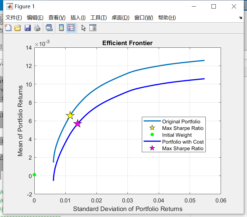
Fig. 1. Efficient frontier of MV and MVC models in first week.

For the second week, we use the previous maximum Sharpe Ratio point as the initial point and continue the method. Because the initial weight is not far from the second maximum Sharpe Ratio point, it is covered by the sign of it. Due to the transaction cost, the efficient frontier of MVC model is not that smooth like MV model, there is a turning point on it.

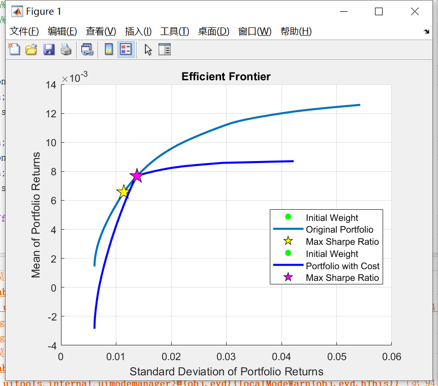
Fig.2. Efficient frontier of MV and MVC models in second week.

The MVCT in Fig.3 with 20% turnover is much smaller than the MVC. As the MVC can be seen as the turnover is 100%. The maximum Sharpe Ratio of the two models are the same, as they are just on the overlap and the turnover don’t affect the maximum Sharpe Ratio.

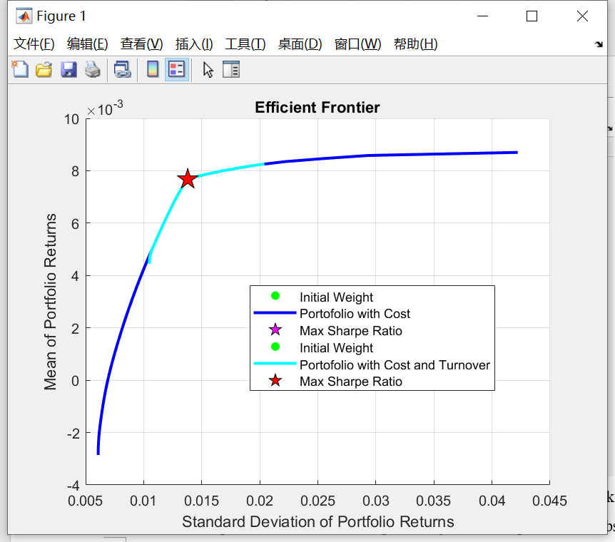
Fig.3. Efficient frontier of MVC and MVCT models in second week.

Then we draw the graphs of different turnovers to find the difference between them. Fig.4 demonstrates that the smaller the turnover rate, the shorter the efficient frontier and the closer it is to the initial weight. Because it can just be changed a little compared with the previous portfolio with a small turnover. When the turnover is equal to 0, the efficient frontier will just be a point on initial point.

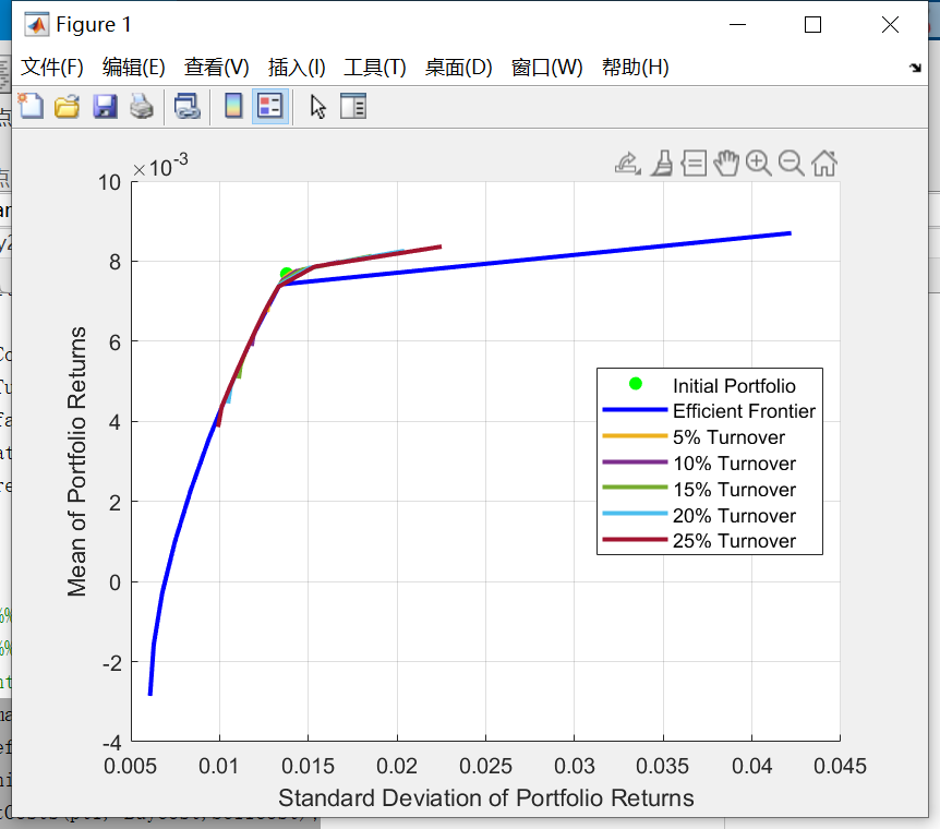
Fig.4. Efficient frontier of MVCT models with different turnover in second week.

For the third week, Fig.5 seems similar to Fig.2, Fig.6 seems similar to Fig.3, as the process will level off over time.

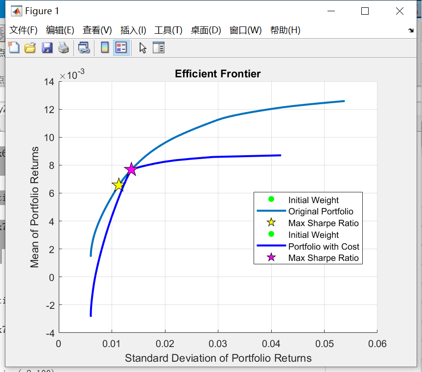
Fig.5. Efficient frontier of MV and MVC models in third week.

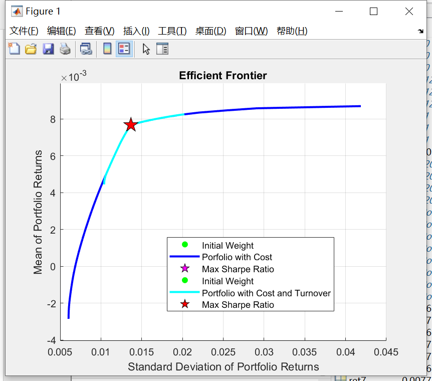
Fig.6. Efficient frontier of MVC and MVCT models in third week.

However, Fig.7 is also similar to Fig.4. It just be enlarged to better observe the difference in different turnovers. It exactly shows that the smaller the turnover rate, the closer the line is to the original weight.

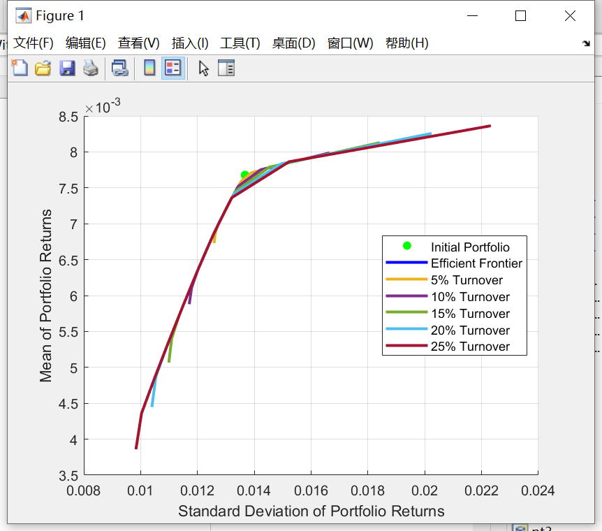
Fig.7. Efficient frontier of MVCT models with different turnover in third week.

Table 1 shows the patterns of the three models more clearly. Combined with previous figures analysis, the MVC model is more volatile than the MV model. The MVC model and MVCT model with 20% turnover are same in the optimal point, owning to the second week and third week changing weights do not exceed 20%.

Table 1. Maximum Sharpe Ratio point in each models.

5 Discussion

From Fig.1, Fig.2, and Fig.5, it showed the MV and MVC models at different times. Both of them showed that when adding the transaction cost in MV model, the model will shift down to the right. Compared with the classical MV model, it will spend money when the trade happens. Obviously, the return will decrease because of it. And the MVC curve in the second and third week had the turning point, where the MV and MVC overlapped. After the turning point, the curve became placid in week 2 and week 3. This is due to the more trading carried out than in week 1, the more transaction cost with less return and higher volatility there will be. And the turning point in the next two weeks is exactly the max Sharpe Ratio point. However, the point in week 1 has nearly the same standard deviation but different rate. It showed that the investor first bought the different weight of stock, and held it for the next two weeks. So, the volatility had little change, but the next two weeks had 0.002 higher return with no transaction cost in the next two weeks.

From Fig.3 and Fig.6, the MVCT curve is shorter than MVC. The MVC model can be resembled as the MVCT model with 100% turnover. The week 1’s turnover is 100% on account of first buying stocks must be 100%. Thus, the turnover constraint carried out in week 2. And the previous max Sharpe Ratio as the next initial weight of the portfolio. So, when the turnover rate is 20%, the turnover didn’t change the max Sharpe Ratio rate. Fig.4 and Fig.7 showed that with smaller turnover, the curve is shorter, the closer the line is to the original weight. When the turnover rate is 0%, the weight of stocks stayed the same as the previous week.

The research was only carried out 3 weeks, from Table 1 the data of the three models became stable in week 3. And if we still simulate the data in week 4 or later, the weight won’t change a lot. Moreover, with the time increasing, the timeliness and validity of previous data decreases.

6 Conclusion

On the basis of Markowitz's model, this paper modifies the model according to the actual Chinese market, adding restrictions on transaction costs and turnover rate, and conducts a comparative study on the three models before and after modification. With the addition of new variables, the modified model expands the scope of the study from one point in time to one time period. It is found that the addition of transaction costs makes the Efficient Frontier move to the right and down, while the restriction of turnover rate has no effect on the maximum Sharp Ratio point, because the maximum Sharp Ratio point at each time point is not far apart. This paper puts forward further optimization for the practical application of Markowitz model in the Chinese market, so as to make it more effective in the practical application of portfolio construction.

The main limitation of the study in this paper is that the lag time of the model cannot be extended. The model tends to be stable after 3 time points, and the deviation of the prediction data model in the future is too large. According to my research, the future research direction can start from several classical assumptions of the Markowitz model, modify those assumptions that are not suitable for practical application, and optimize the model.

References

[1]. Markowitz, H. (1952).Portfolio selection. The Journal of Finance,7(1),77–91.
[2]. Markowitz, H. (1959).Portfolio Selection, Efficient Diversification of Investments. J. Wiley
[3]. Kulali, I. (2016). Portfolio optimization analysis with Markowitz quadratic mean-variance model. European Journal of Business and Management, 8(7), 73-79.
[4]. Ivanova, M., & Dospatliev, L. (2017). Application of Markowitz portfolio optimization on Bulgarian stock market from 2013 to 2016. International Journal of Pure and Applied Mathematics, 117(2), 291-307.
[5]. de Melo Neto, J. J., & Fontgalland, I. L. (2022). Share portfolio advisory: Use of the Markowitz method to optimize the risk/return ratio in individual investor shares portfolio. Research, Society and Development, 11(2), e26011225921-e26011225921.
[6]. Li J, Peng Y, & Cao XZ. (2017). Research on the optimal investment portfolio of corporate annuities based on investment constraints. Financial Theory and Practice (7), 4.
[7]. Li, Shu-Li. (2020). A study of Markowitz portfolio model with mean and variance changes. Bohai Rim Economic Outlook (2), 2.
[8]. Iqbal, J., Sandhu, M. A., Amin, S., & Manzoor, A. (2019). Portfolio Selection and Optimization through Neural Networks and Markowitz Model: A Case of Pakistan Stock Exchange Listed Companies. Review of Economics and Development Studies, 5(1), 183-196.
[9]. Yu, H.& Li, L.(2013). Markowitz’s Portfolio Model and Its Empirical Research Based on Security Market in China. Journal of Gansu Sciences,25(3),146–149.
[10]. Altman, E. I., & Saunders, A. (1997). Credit risk measurement: Developments over the last 20 years. Journal of banking & finance, 21(11-12), 1721-1742.
Cite this article
Yang,Y. (2023). Application of Markowitz Model Equipped with Transaction Cost and Turnover Rate in Chinese Stock Market. Advances in Economics, Management and Political Sciences,3,489-496.
Data availability
The datasets used and/or analyzed during the current study will be available from the authors upon reasonable request.
Disclaimer/Publisher's Note
The statements, opinions and data contained in all publications are solely those of the individual author(s) and contributor(s) and not of EWA Publishing and/or the editor(s). EWA Publishing and/or the editor(s) disclaim responsibility for any injury to people or property resulting from any ideas, methods, instructions or products referred to in the content.
About volume
Volume title: Proceedings of the 6th International Conference on Economic Management and Green Development (ICEMGD 2022), Part Ⅰ
© 2024 by the author(s). Licensee EWA Publishing, Oxford, UK. This article is an open access article distributed under the terms and
conditions of the Creative Commons Attribution (CC BY) license. Authors who
publish this series agree to the following terms:
1. Authors retain copyright and grant the series right of first publication with the work simultaneously licensed under a Creative Commons
Attribution License that allows others to share the work with an acknowledgment of the work's authorship and initial publication in this
series.
2. Authors are able to enter into separate, additional contractual arrangements for the non-exclusive distribution of the series's published
version of the work (e.g., post it to an institutional repository or publish it in a book), with an acknowledgment of its initial
publication in this series.
3. Authors are permitted and encouraged to post their work online (e.g., in institutional repositories or on their website) prior to and
during the submission process, as it can lead to productive exchanges, as well as earlier and greater citation of published work (See
Open access policy for details).