1. Introduction

Markowitz introduced the Mean-Variance model, which revolutionized portfolio optimization by considering both the expected returns and the risk associated with different asset allocations [1]. This seminal work laid the foundation for modern portfolio theory and become a focus of modern finance.

Since then, numerous research papers have focused on refining and extending the Mean-Variance model. Das et al. introduce a novel approach to portfolio management that incorporates psychological factors and the concept of mental accounting, allowing investors to make more informed and personalized investment decisions [2]. Over time, there has been a surge in enthusiasm for the application of state-of-the-art methodologies [3]. Furthermore, Laher et al. explores the use of deep learning models, including GRU and LSTM, for the optimization of portfolio rebalancing, contributing to the advancement of machine learning techniques in the field of finance [4]. In a subsequent study, Kisiel et al. introduce the innovative use of attention-based models, such as the Portfolio Transformer, to improve the effectiveness of asset allocation strategies [5]. However, there is still a lack of relevant research in this area, so this paper aims to further explore the optimization of portfolios using four deep learning methods.

By leveraging deep neural networks and self-attention mechanism, the paper presents an approach for portfolio optimization and contributes to the development of advanced techniques for optimizing investment portfolios using deep learning methods. To test the proposed methods, a selection of five representative stocks from the U.S. stock market was made. In order to train each model, the study employed weekly stock price data from the preceding 52 weeks to forecast the subsequent week's stock prices. Subsequently, the mean-variance optimization method was employed to determine optimal portfolio weights on a weekly basis. Throughout the test dataset, this process was repeated for each week, with portfolio weights being updated based on the most recent real stock prices. Upon completion of the testing period, the overall portfolio returns were computed and compared against the returns generated by the SP500 index as a benchmark [6].

The paper is organized as follows: Section 2 presents a detailed description of the data utilized in this research and discusses the methodology employed for stock selection, accompanied by a descriptive analysis of the chosen stocks. Section 3 elaborates on the methods employed in this research, providing detailed explanations. In Section 4, the effectiveness of the proposed approach is examined, comparing it to benchmark assets and other simplistic portfolios. Finally, Section 5 concludes the paper, highlighting key findings and suggesting potential directions for future research.

2. Data and Methodology

2.1. Data Source and Pre-process

This paper carefully selects 5 representative stocks based on several key factors. Firstly, emphasis is placed on identifying industry leaders that drive technological advancements and innovation. These stocks represent companies at the forefront of their respective sectors, showcasing their ability to shape and influence industry trends. Secondly, the selection process takes into account the financial performance of the chosen stocks, prioritizing companies with a track record of consistent growth, profitability, and efficient operations. The selected stocks are listed in Table 1 as follows:

Table 1: Selected stocks.

The study collected the adjusted closing prices of five stocks from July 2nd, 2013, to July 2nd, 2023, from Yahoo Finance (https://finance.yahoo.com/). Subsequently, the dataset was partitioned into a training set and a test set. The study performed data cleaning to align the timestamps. In total, the study obtained 523 data points for further research. The reason for selecting stock prices from the past decade for research is to analyze recent market trends and incorporate up-to-date information for more relevant insights. Table 2 and Figure 1 presents the descriptive statistics for five stocks. These statistics provide a concise summary of the data distribution and variability, offering insights into the average performance, range, and dispersion of stock prices for the selected stocks.

Table 2: Descriptive statistics of five stocks.

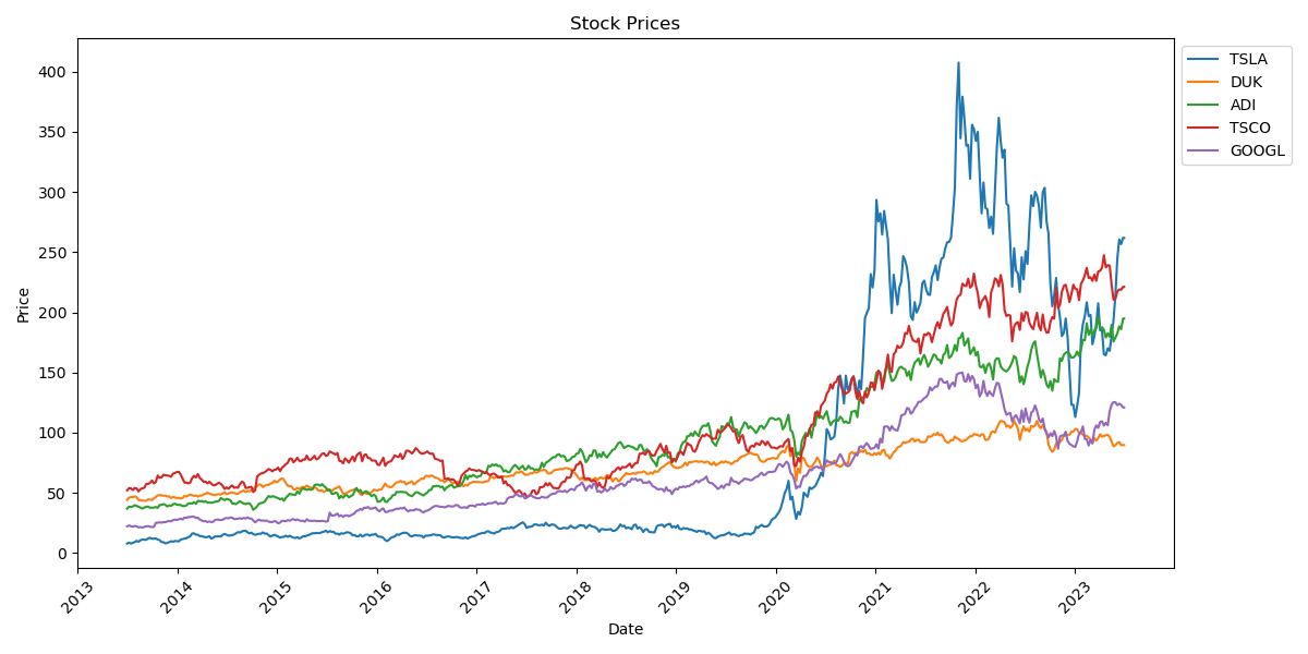
Figure 1: Weekly price of selected stocks.

2.2. Long Short-Term Memory (LSTM)

LSTM is a specialized recurrent neural network that addresses the challenge of capturing long-term dependencies [7]. It introduces a cell state \( {c_{t}} \) and three gates: the forget gate \( {f_{t}} \) , input gate \( {i_{t}} \) , and output gate \( {o_{t}} \) . These gates control the flow of information and help the model retain important contextual information over extended sequences. By overcoming the vanishing gradient problem, LSTM has become a powerful tool in various domains.

2.3. Gated Recurrent Unit(GRU)

GRU is a variant of the LSTM model that simplifies its architecture by using only two gates: the reset gate \( {r_{t}} \) and the update gate \( {z_{t}} \) [8]. These gates play a crucial role in determining the behavior of the hidden state \( {h_{t}} \) . The reset gate controls how the current input is combined with the historical memory, while the update gate determines the extent to which the historical memory is retained in the node. By training the weights of the reset and update gates through backpropagation, the GRU model can effectively capture and utilize both short-term and long-term dependencies in the input sequence.

2.4. Self-Attention

The self-attention mechanism provides the advantage of capturing long-range dependencies and identifying relevant features in stock prediction tasks [9]. This abstraction highlights the selective focus on relevant information and the dynamic allocation of attention. It enables the model to capture important features by assigning varying weights to different values, regardless of the specific framework used.

In the initial phase, the weight coefficients associated with each Key, corresponding to the given Value, are determined by evaluating the relevance between each Query and the Keys. In this context, K represents the Key, Q represents the Query, F denotes a function, V signifies the weight value, Sim denotes similarity, a represents the weight coefficient, and A represents the attention value. These calculations determine the attention weights assigned to different Key-Value pairs, allowing the model to selectively focus on relevant information. This flexibility in computing the attention coefficients enables the model to adapt to different scenarios and capture important features effectively.

In the second phase, the weights are normalized using a function similar to SoftMax, as shown in Equation (13).

In the third stage, the attention values are computed by taking the weighted sum of the attention weights ( \( {a_{i}} \) ) and the corresponding values ( \( {V_{i}} \) ), as shown in Equation (14). This step combines the relevance of each key-value pair to generate the final attention value.

2.5. Transformer

The Transformer model has the advantage of capturing long-range dependencies and effectively modeling sequential data, making it well-suited for predicting stock prices [10]. The Transformer model adopts an encoder-decoder architecture to effectively capture global dependencies between the input and output using attention mechanisms. Unlike traditional recurrent structures, it eliminates the need for recursion and achieves efficient parallel processing of data. The encoder is composed of six identical layers, which consist of a multi-head attention layer and a feed-forward layer. In contrast, the decoder has a more complex architecture that includes masked multi-head attention layers. By employing self-attention mechanisms, the Transformer model effectively preserves long-distance information between data and enhances the efficiency of training.

The Transformer architecture utilizes linear transformations of the input data to derive the matrix of queries (Q), the matrix of keys (K), and the matrix of values (V), with computations following the formulas.

These parameters matrices ( \( W_{i}^{Q},W_{i}^{k},W_{i}^{v} \) ) are utilized to apply linear transformations to the input data.

2.6. Mean-Variance (MV)

MV model offers a mathematical framework for determining the optimal weights assigned to each asset in an investor's portfolio. The MV model aims to maximize portfolio returns while considering the associated level of risk. Let \( {w_{i}} \) represent the weight assigned to the i-th asset, satisfying the constraint \( \sum _{i}{w_{i}}=1 \) , and \( {μ_{i}} \) denote the anticipated yield of the i-th asset. The expected returns of the portfolio can then be expressed as follows, where R_p signifies the overall expected portfolio return:

Denote \( {σ_{i}} \) as the standard deviation of the \( i \) -th asset and \( {ρ_{ij}} \) as the correlation between the returns of the \( i \) -th and \( j \) -th asset. Then the portfolio return variance is

Ideal portfolios lie on the efficient frontier. The equations can be transformed into matrix form, making implementation and efficient frontier calculations more convenient. The objective function for the Mean-Variance (MV) model is expressed as:

In the Mean-Variance (MV) model, the portfolio weights vector, denoted by w, and the sample covariance matrix of asset returns, denoted by Σ, play crucial roles. The sample covariance matrix represents the historical data used for computation. To enhance the performance of the covariance matrix, certain adjustments can be made. The parameter q quantifies the investor's risk tolerance.

Two portfolios of particular interest in the MV model are the minimum volatility portfolio and the maximum Sharpe ratio portfolio (MSP). The minimum volatility portfolio (MVP) corresponds to q=0, indicating complete risk aversion by the investor. The Sharpe ratio is a widely used measure for evaluating risk-adjusted return. It is calculated as follows:

where \( {R_{f}} \) is the current risk-free rate of the market.

3. Results

The study initially assessed the fitting performance of GRU, LSTM, Self-Attention, and Transformer models MSE as the evaluation metric. Each model was trained for 10 epochs. Through extensive parameter tuning, the study obtained predictions for asset prices using these four models. Notably, the models demonstrated a certain level of accuracy in predicting future values of the asset price, as evidenced by the close alignment observed between the predictions and the validation values of the test set. The following Table 3 presents the mean squared error (MSE) values for each company corresponding to the four models:

Table 3: MSE for each corporation-model pair.

This study proposes a trading strategy based on a weekly time frame. Throughout the 52-week testing period, the asset weights for each week are determined using the predictions generated by four distinct models: GRU, LSTM, Self-Attention, and Transformer. Each model corresponds to a set of weights that are utilized to construct portfolio strategies aimed at maximizing the Sharpe ratio and minimizing the variance. As a result, a total of eight portfolio strategies are developed, representing different combinations of the predictive models and optimization objectives.

To assess the performance of each model, the study obtains the historical returns of the S&P 500 index during the test period as a benchmark for the market. Subsequently, an ex-post analysis is conducted to determine the actual returns of each portfolio. The weights presented in Table 4 represent the allocations of the five companies for each respective model during the initial week, while Figure 2 illustrates the cumulative returns of each portfolio over time.

Table 4: Initial Week Weights.

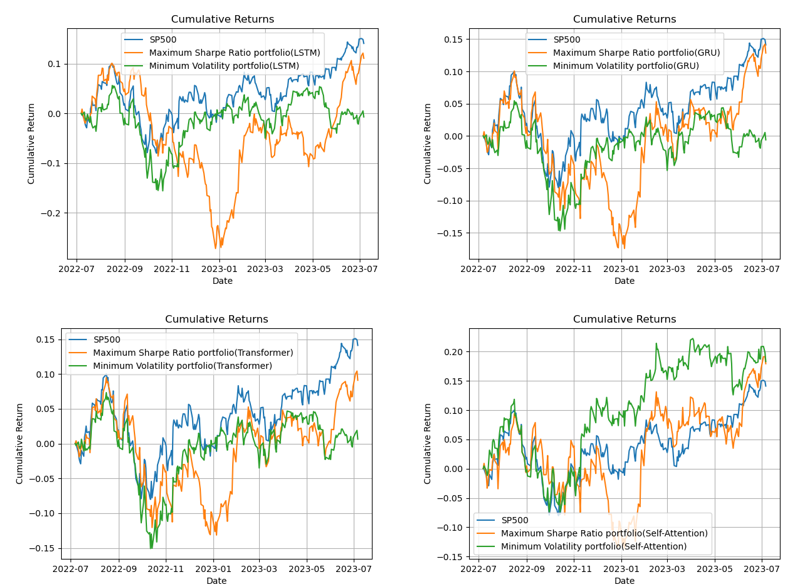
Figure 2: Comparison between SP 500 returns and alternative portfolios.

Based on the findings, the following characteristics can be observed:

The cumulative returns of the two combinations (MVP, MSP) corresponding to LSTM, GRU, and Transformer models are lower than the cumulative return of the S&P 500 index (14.2%); The cumulative returns of the two combinations (MVP, MSP) corresponding to the self-attention model (18.3%, 18.0%, respectively) were slightly higher than the cumulative return of the benchmark(14.2%); The cumulative returns of the benchmark are more stable compared to the cumulative returns of the MSP and MVP portfolios corresponding to each model; The target model (MVP corresponding to Self-Attention) has consistently outperformed both the S&P 500 and MSP corresponding to Self-Attention since November 2022. Furthermore, it has exhibited greater stability compared to the MVP portfolio, indicating a more consistent and favorable performance.

4. Conclusion

Deep learning techniques have revolutionized portfolio optimization in the finance domain, offering new perspectives and opportunities. This study focuses on the selection of stocks from Google, Tesla, Tractor Supply Company, Analog Devices, and Duke Energy Corporation. Leveraging the power of four deep learning models, returns and covariance estimates are derived for these stocks, respectively. The mean-variance model is then utilized to construct target portfolios for each deep learning model, incorporating the predicted outcomes. Subsequently, a comparative analysis is conducted between the returns of these portfolios and the market benchmark. The findings unveil the superior performance of our proposed target model across various financial metrics, indicating its potential for innovative portfolio allocation strategies. This research sheds light on the groundbreaking and promising applications of deep learning in the financial sector, paving the way for advancements in portfolio optimization through the integration of deep learning methodologies.

GRU, LSTM, Self-Attention, and Transformer models have proven effective in predicting stock prices. However, they do have limitations. These models may struggle to capture abrupt market changes and unpredictable events. They can be sensitive to extreme market conditions and outliers, impacting their accuracy. Additionally, overfitting can occur when the models are trained on limited or noisy data. Another challenge is their lack of interpretability, as they operate as complex black-box models. Despite these limitations, these models offer valuable insights and can be enhanced by addressing their weaknesses and combining them with other approaches in stock price prediction.

References

[1]. Markowitz, H. (1952) Portfolio Selection. The Journal of Finance, 7(1), 77–91.
[2]. Das, S., Markowitz, H., Scheid, J., and Statman, M. (2010) Portfolio optimization with mental accounts. Journal of financial and quantitative analysis, 45(2), 311-334.
[3]. Ma, Y., Han, R., and Wang, W. (2021) Portfolio optimization with return prediction using deep learning and machine learning. Expert Systems with Applications, 165, 113973.
[4]. Laher, S., Paskaramoorthy, A., and Van Zyl, T. L. (2021). Deep learning for financial time series forecast fusion and optimal portfolio rebalancing. In 2021 IEEE 24th International Conference on Information Fusion, 1-8.
[5]. Kisiel, D., and Gorse, D. (2022). Portfolio transformer for attention-based asset allocation. In International Conference on Artificial Intelligence and Soft Computing, 61-71.
[6]. Bailey, J. V. (1992) Evaluating benchmark quality. Financial Analysts Journal, 48(3), 33-39.
[7]. Schmidhuber, J., and Hochreiter, S. (1997) Long short-term memory. Neural Comput, 9(8), 1735-1780.
[8]. Cho, K., Van Merriënboer, B., Gulcehre, C., Bahdanau, D., Bougares, F., Schwenk, H., and Bengio, Y. (2014) Learning phrase representations using RNN encoder-decoder for statistical machine translation. arXiv preprint arXiv:1406.1078.
[9]. Hu, Y., and Xiao, F. (2022) Network self attention for forecasting time series. Applied Soft Computing, 124, 109092.
[10]. Zhou, T., Ma, Z., Wen, Q., Wang, X., Sun, L., and Jin, R. (2022) Fedformer: Frequency enhanced decomposed transformer for long-term series forecasting. In International Conference on Machine Learning, 27268-27286.
Cite this article
Zhang,E. (2023). Portfolio Optimization Strategy Based on Four Deep Learning Models. Advances in Economics, Management and Political Sciences,47,295-302.
Data availability
The datasets used and/or analyzed during the current study will be available from the authors upon reasonable request.
Disclaimer/Publisher's Note
The statements, opinions and data contained in all publications are solely those of the individual author(s) and contributor(s) and not of EWA Publishing and/or the editor(s). EWA Publishing and/or the editor(s) disclaim responsibility for any injury to people or property resulting from any ideas, methods, instructions or products referred to in the content.
About volume
Volume title: Proceedings of the 2nd International Conference on Financial Technology and Business Analysis
© 2024 by the author(s). Licensee EWA Publishing, Oxford, UK. This article is an open access article distributed under the terms and
conditions of the Creative Commons Attribution (CC BY) license. Authors who
publish this series agree to the following terms:
1. Authors retain copyright and grant the series right of first publication with the work simultaneously licensed under a Creative Commons
Attribution License that allows others to share the work with an acknowledgment of the work's authorship and initial publication in this
series.
2. Authors are able to enter into separate, additional contractual arrangements for the non-exclusive distribution of the series's published
version of the work (e.g., post it to an institutional repository or publish it in a book), with an acknowledgment of its initial
publication in this series.
3. Authors are permitted and encouraged to post their work online (e.g., in institutional repositories or on their website) prior to and
during the submission process, as it can lead to productive exchanges, as well as earlier and greater citation of published work (See
Open access policy for details).