


1. Introduction
Portfolio is not a new concept in the financial world. Since the age of Shakespeare, the concept of diversification was well-established [1]. Despite the fact that the diversification of services and risks is a nature of portfolio selection, it was not until 1952 that the topic was academically elaborated by Markowitz [2]. However, after years of development, it is not exaggerated to say that modern portfolio theory has brought revolutions to the investment management world, largely thanks to its power to achieve the maximum return while maintain the lowest entire risk [3].
In the past decade, efforts have been made to continuously improve the portfolio selection. In research conducted by DeMiguel and several other researchers, positive effects of statistical information of stock prices on constructing the optimal portfolio are observed [4]. The research indicates that taking option-implied volatility and skewness into consideration when using models to predict future performance can significantly reduce volatility and increase Sharpe ratio. Machine learning is also widely used in the field. For instance, the support vector machine (the SVM method) has been used in one research to produce forecasting results of stocks [5]. The result is then combined with another mean variance model to fit test data to calculate the optimal portfolio. Apart from the SVM method, various optimizing methodologies can be used to do similar forecasting. Another research proves performance-based regularization (PBR) as the solution to both mean-variance problems and mean-conditional value-at-risk problems are effective (CVaR) [6]. Counterintuitively, it is not always the case that a more complex model necessarily performs better than a relatively simpler model in forecasting. As illustrated by Ghandar and two other researchers, they in fact observe more sophisticated models underperform simpler models in forecasting out-of-sample data [7]. Even though a relatively precise model is chosen, there is always the potential risk of overfitting when performing forecasting tasks using the model [8]. What is more, the portfolio theory is also highly possible to be influenced by domestic government policies, just as illustrated by Wang [9]. Despite the versatility of predicting models, LSTM models seem to be considerably successful. As illustrated in one research, LSTM models help achieve a 50% increase in annualized return [10]. However, there are few research focus on the capability of LSTM models combined with rather simple optimizing strategies earning considerable return in shorter period.
The main purpose of the paper is mainly to evaluate the effectiveness of the combination of long-short term memory models and minimizing variation portfolio optimization in solving portfolio optimizing problems. To achieve the purpose, 11 stocks are chosen separately from 11 industries as portfolio 1. For further discussion, another 10 stocks are chosen as portfolio 2. Daily adjusted close prices are chosen as the input of LSTM models in the hope to allow the model to grasp the most information. After forecasting the expected prices of the 11 stocks, a covariance matrix can be constructed accordingly. Finally, the optimizing strategy of achieving minimum portfolio variation used to find the optimal portfolio. The whole process would say something about whether LSTM forecasting and the minimal variation optimization is a relatively universal and well-performed method in real world market. It would also provide validation to the statement regarding the relationship between the complexity of a model and its actual performance. What is more, it also gives some hints regarding real world stock trading strategies.
The structure of this paper is as below. Data section will include standards used to filter out 11 stocks and exact figures. Methods section will mainly introduce the LSTM model and covariance matrix. In the result section, two optimal portfolios and their expected returns will be given and evaluated. There is also a sub-section of further discussions about the result. Some implications of the result will also be introduced in this section. Finally, the last section is a conclusion to the whole study and possible future research suggestions.
2. Data
The research will only focus on the stocks listed in the American market. Two groups of data are selected separately under different standards. According to the global industry classification standard (GICS), the market is classified into 11 industries [11]. As illustrated by Fabozzi and two other researchers, the less stocks are correlated, the better the portfolio expected return will be [12]. From this start point, 11 stocks are chosen respectively from 11 different industries. The stocks filtering process for the first group of data is completed following steps below.
Daily adjusted closed prices of stocks in 11 industries from 01/01/1990 to 06/16/2023 on Yahoo Finance are collected with the help of the Pandas package. A sorted list is produced for each industry, ranking the according stocks from the highest Sharpe ratio to the lowest. A second factor of the length of data set is taken into consideration. As a matter of fact, some stocks are listed on the Nasdaq later than some other stocks, leading to the potential problem of lacking sufficient data to train the model. To avoid such scenario, stocks that are in the top 5 list of each industry but have significantly shorter listing span are ruled out.
The portfolio of Warren Buffett is selected as the base of the second group of data as counterpart group. By analyzing the percentage of each stock in his portfolio, top 10 stocks are selected, which already make up of over 90% of Buffett’s total portfolio [13].
A statistical analysis was performed to all stocks used in the research, and the results are presented in Table 1 sorted by the stock code from A to Z.
Table 1: Statistical analysis of 21 stocks.
Stock Code | Mean | Standard Deviation | Skewness | Kurtosis |
AAPL | 17.29 | 37.57 | 2.81 | 7.13 |
ATVI | 21.20 | 26.93 | 1.32 | 0.34 |
AXP | 31.61 | 40.56 | 1.75 | 2.70 |
BAC | 12.31 | 11.62 | 0.81 | -0.43 |
BNTX | 136.47 | 81.68 | 0.91 | 0.76 |
CHRD | 30.25 | 38.01 | 1.82 | 2.13 |
CVX | 25.95 | 36.55 | 1.70 | 2.52 |
HPQ | 5.96 | 7.51 | 1.59 | 2.47 |
KHC | 43.37 | 14.49 | 0.37 | -1.17 |
KO | 12.06 | 15.45 | 1.41 | 1.26 |
LAC | 6.81 | 7.85 | 1.87 | 2.53 |
MA | 127.91 | 123.65 | 0.85 | -0.81 |
MCO | 77.62 | 95.14 | 1.65 | 1.65 |
MNST | 9.03 | 14.34 | 1.59 | 1.34 |
NFE | 27.67 | 13.18 | 0.143 | -1.25 |
NFLX | 124.83 | 169.13 | 1.355 | 0.64 |
NSA | 28.00 | 13.56 | 0.77 | -0.30 |
OXY | 24.05 | 24.15 | 0.66 | -1.23 |
SHOP | 42.36 | 44.93 | 1.18 | 0.16 |
TDG | 214.06 | 218.57 | 0.97 | -0.37 |
TSLA | 63.13 | 96.69 | 1.66 | 1.38 |
For data of each stock, 80% of the total data is selected as the train group, 10% of the total data is selected as the validation group, and the final 10% is the test data. Individua LSTM model is trained based on the train data. Then, the optimal model is fitted into the validation group to check whether the model is effective to do forecasts. Finally, the model was fitted to the test group to make the next 21-day forecasts.
3. Method
3.1. The Ex Ante Sharpe Ratio
Sharpe Ratio is a widely used tool in the financial world. It reveals the ability of a financial asset retaining extra benefit given a certain risk rate. Sharpe illustrated the idea of the Ex Ante Sharpe Ratio thoroughly [14]. The equation for it is shown below.
\( S = \frac{{R_{F}}-{R_{B}}}{{σ_{F}}} \) | (1) |
In the equation above, \( {R_{F}} \) stands for the return of a given stock F, while \( {R_{B}} \) stands for the return of a given benchmark financial asset B. \( {R_{F}}-{R_{B}} \) .stands for the standard deviation of the differential return \( {σ_{F}} \) .
In the particular research, the Ex Ante Sharpe Ratio is mostly used in the data section. \( {R_{F}} \) is the return of any given stock in one of the 11 industries. \( {R_{B}} \) , the return of a benchmark financial assets, or risk-free rate.
3.2. Long Short-Term Memory
The Long Short-Term Memory (LSTM) was first introduced by Hochreiter and Schmidhuber in 1997 [15]. The innovative method concurs the obstacle facing by traditional RNN network capturing long-term dependencies in data and manages to find an equilibrium between long-term historical data and new data. The LSTM used in the research can be mathematically expressed as below.
\( {F_{t}}=σ({W_{f}}[{X_{t}}, {H_{t-1}}]+{b_{f}}) \) | (2) |
\( {I_{t}}=relu({W_{i}}[{X_{t}}, {H_{t-1}}]+{b_{i}}) \) | (3) |
\( \widetilde{{C_{t}}}=tanh({W_{c}}[{X_{t}}, {H_{t-1}}]+{b_{c}}) \) | (4) |
\( {C_{t}}={F_{t}}*{C_{t-1}}+{I_{t}}*\widetilde{{C_{t}}} \) | (5) |
\( {O_{t}}=linear({W_{o}}[{H_{t}}, {C_{t}}]+{b_{o}}) \) | (6) |
\( {H_{t}}={O_{t}}tanh({C_{t}}) \) | (7) |
Equation 2 is the mathematical expression for the forget gate of LSTM. Equation 3 is the mathematical expression for the input gate. Equation 4 represents the candidate cell state. Equation 5 represents the new cell state. Equation 6 is the mathematical expression for the output gate. Equation 7 represents the hidden state. \( σ, relu, tanh, linear \) are 4 different activation functions used in LSTM. \( {W_{f}}, {W_{i}}, {W_{c}}, {W_{o}} \) represent the weight matrix for the according gate.
3.3. Minimal Variation Optimization
The minimal variation optimization is a technique designed to find the optimal weight for a portfolio achieving the minimal variation using covariance matrix. Denote \( w=[{w_{1}}, {w_{2}}, …, {w_{3}}] \) as a vector of weights representing the proportion of each asset in the portfolio. The portfolio expected return is denoted as \( E(R)=w.T @ μ \) , and \( μ=[{μ_{1, }} {μ_{2}},…, {μ_{n}}] \) represents a vector of expected returns for each asset. The risk of the portfolio is denoted as \( {σ^{2}}=w.T @ σ @ w \) , where \( σ \) represents a covariance matrix of the stock returns. The Markowitz portfolio optimization problem can then therefore be denoted as below.
\( Minimize: {σ^{2}} \) | (8) |
\( Subject to:w.T @ 1=1, w≥0 \) | (9) |
This formulation seeks to minimize the variance of the portfolio subject to the constraints that the weights sum to 1 and are non-negative. The optimal weights obtained from solving this optimization problem will provide the portfolio with the lowest risk for a given set of assets.
4. Result
4.1. Portfolio 1
The LSTM successfully capture the changes in the price of stocks chosen. Train group, validation group, and the test group are selected as mentioned in the data section. The individual LSTM model is evaluated. The results are shown in Table 2.
Table 2: LSTM evaluation of portfolio 1.
MSE | RMSE | MAE | |
BNTX | 151.95 | 12.33 | 11.82 |
CHRD | 20.91 | 4.57 | 3.79 |
LAC | 0.64 | 0.80 | 0.58 |
MSE | 44.88 | 6.70 | 5.43 |
MNST | 58.49 | 7.65 | 7.25 |
NFE | 81.48 | 9.03 | 8.94 |
NFLX | 3005.98 | 54.83 | 50.20 |
NSA | 66.69 | 8.17 | 7.99 |
SHOP | 16.88 | 4.11 | 3.82 |
TDG | 2918.87 | 54.03 | 50.68 |
TSLA | 3788.57 | 61.55 | 58.53 |
The optimal LSTM model for each stock is chosen under the method of adaptive moment estimation (Adam) with a learning rate of 0.0001, and the loss function for the method is the mean squared error. The process was repeated for 30 times. Then the optimal LSTM model is fitted to the last 21 entries in the test group one for each time. This process results in a forecasting result of 21 days. Based on the forecasting result, a covariance matrix is constructed. The optimization objective is to minimize risks. The optimal weight for each stock is shown in Table 3.
Table 3: Optimal weight of portfolio 1
BNTX | CHRD | LAC | MA | MNST | NFE |
7.74% | 11.41% | 10.85% | 13.59% | 17.78% | 12.19% |
NFLX | NSA | SHOP | TDG | TSLA | |
0 | 0% | 11.78% | 7.36% | 7.31% |
Based on the weight optimized by LSTM forecasting and the real-world daily return of 11 stocks, the portfolio return can be calculated as shown in Figure 1.
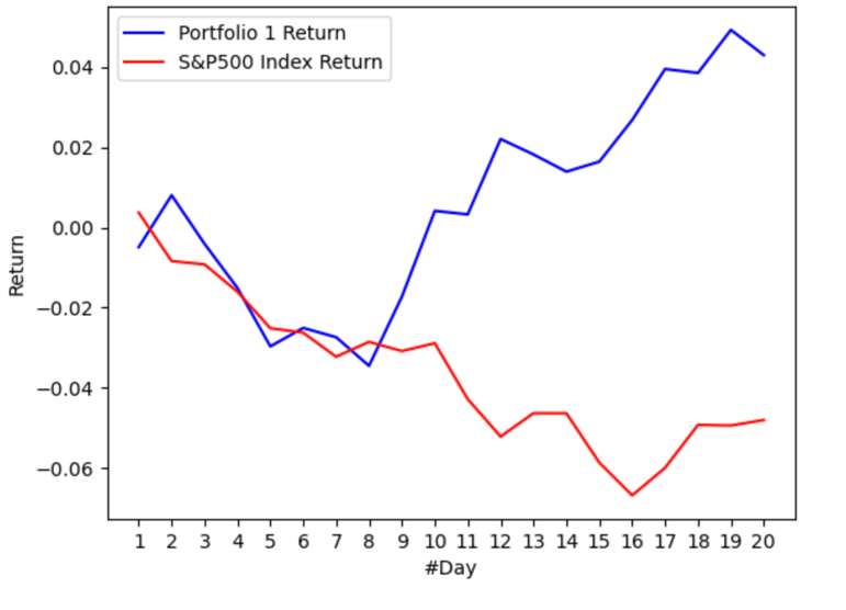
Figure 1: Portfolio 1 return vs S&P500 index return.
The portfolio 1 return and the S&P500 index return are first synchronous, showing downward trending. However, after the 8th day, two returns in question move toward completely opposite directions. The portfolio 1 return turns over to overall-all increasing, while the S&P500 index remain the decreasing trend. In the 20th day, the portfolio 1 achieves a return of 4.29%. On contrary, the return of S&P500 index is -4.8%.
Overall speaking, the result of portfolio 1 optimization is quite promising. In a time period of 21 trading days, the optimized portfolio clearly beats the market. It certainly proves the method in this research is effective: stocks filtering based on the Sharpe ratio and the data length, LSTM forecasting, and portfolio construction using forecasting result of LSTM.
4.2. Portfolio 2 and Further Discussion
The same process is performed to the counterpart. The individual LSTM model is evaluated. The result is shown in Table 4.
Table 4: LSTM evaluation of portfolio 2.
MSE | RMSE | MAE | |
AAPL | 7189.92 | 84.79 | 82.64 |
ATVI | 3.17 | 1.78 | 1.40 |
AXP | 1446.93 | 38.04 | 32.12 |
BAC | 1.15 | 1.07 | 0.94 |
CVX | 481.48 | 21.94 | 20.06 |
HPQ | 32.31 | 5.68 | 5.20 |
KHC | 1.21 | 1.10 | 0.93 |
KO | 73.51 | 8.57 | 8.05 |
MCO | 679.09 | 26.06 | 24.76 |
OXY | 0.52 | 0.72 | 0.61 |
The optimal weight for each stock is shown in Table 5.
Table 5: Optimal weight of portfolio 2.
AAPL | ATVI | AXP | BAC | CVX |
0 | 8.11% | 0 | 29.72% | 0 |
HPQ | KHC | KO | MCO | OXY |
0 | 20.67% | 0 | 2.23% | 39.25% |
Based on the weight optimized by LSTM forecasting and the real-world daily return of 10 stocks, the portfolio return can be calculated as shown in Figure 2.
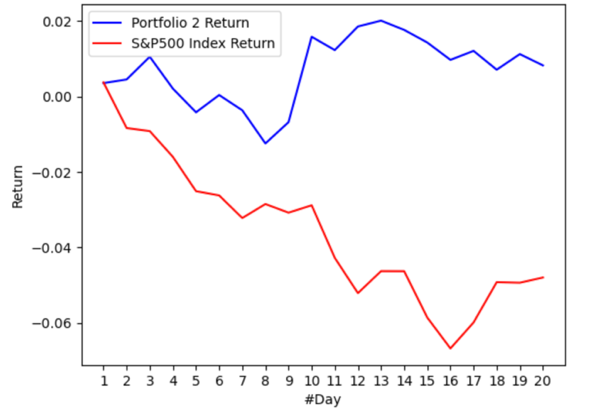
Figure 2: Portfolio 2 return vs S&P500 index return.
The portfolio 2 return and the S&P500 index return are also first synchronous in the term of moving trend. Similar to what happened in portfolio 1 analysis, starting from the 8th day, the portfolio 2 return begins to move in the opposite direction of S&P500 index return. In the 20th day, the portfolio 2 can achieve a return of 0.82%, while the S&P500 index return is -4.8%. However, it is noteworthy that the portfolio 2 return outperforms the market all the time.
The result of portfolio 2 is not optimistic compared to the result of portfolio 1 as it achieves a lower portfolio return. Various reasons may lead to the gap between the result of portfolio 1 and that of portfolio 2. One direct reason is the robustness of LSTM models. Despite by counts there are more accurate models in portfolio 2 than in portfolio 1, others show dramatic inaccuracy as observed in the model for AAPL. What is more, there is also a trend in both portfolio and portfolio 2 that models for stocks with more data actually are less accurate. Increasing learning rate of Adam or repeating the optimization process for more times may results in more robust models.
Also, the difference in two results also reveals the high volatility of using machine learning to optimize portfolios. Not only the reasons mentioned above may explain the gap, but also the activation function may also lead to different level of accuracy. Besides, different stocks filtering strategies may also lead to different original stocks, and some of these stocks must be more suitable than others for machine learning.
5. Conclusion
The research paper mainly aims to test the effectiveness of the combined method of LSTM forecasting and minimal variation optimizations. LSTM models are constructed to provide forecasting results of the price of 21 stocks in the next 21 days. Based on the forecasting result, covariance matrixes are constructed, and the minimal variance optimization is performed to find the optimal weight for each portfolio. Finally, real-world returns of these 21 stocks are used to calculate the portfolio return for the time period of next 21 days. Portfolio 1 achieves a return of 4.29%, and portfolio 2 achieves a return of 0.82%. By contrast, the S&P500 index return for the same time period is around -4.8%. The result clearly proves that the LSTM enhanced minimal variation optimization is effective in achieve promising returns even during the time when the general market is not optimistic. The research serves as a replicable case for real-world investors to construct their own portfolios.
Overall, the research paper successfully demonstrates the effectiveness of the LSTM enhanced minimal variation optimization in real-world investing cases. However, there are also some aspects that can be further improved. First of all, some of the LSTM models used in the paper are less accurate than others. Secondly, the effectiveness of such method in longer investing time period remains unproved. Finally, some other possible combined methods like LSTM enhanced maximal return optimization are not included in the paper as the initiative of the research is to obtain a promising return under reasonable risks. It is not necessarily the case that maximizing the return will lead to a significant increase in portfolio risks, which means that even under the objective mentioned above, the LSTM enhanced minimal variation optimization may still not be the optimal solution. Future studies may focus on three points listed above to improve the method.
References
[1]. Markowitz, H. (1999) The Early History of Portfolio Theory: 1600–1960. Financial Analysts Journal, 55(4), 5–16.
[2]. Jorion, P. (1992) Portfolio optimization in practice. Financial analysts journal, 48(1), 68-74.
[3]. Fabozzi, F. J., Markowitz, H., and Gupta, F. (2008) Portfolio Selection. Handbook of Finance.
[4]. DeMiguel, V., Plyakha, Y., Uppal, R., and Vilkov, G. (2012) Improving Portfolio Selection Using Option-Implied Volatility and Skewness. SSRN Electronic Journal.
[5]. Paiva, F. D., Cardoso, R. T. N., Hanaoka, G. P., and Duarte, W. M. (2019) Decision-making for financial trading: A fusion approach of machine learning and portfolio selection. Expert Systems with Applications, 115, 635–655.
[6]. Ban, G.-Y., El Karoui, N. and Lim, A.E.B. (2018) Machine Learning and Portfolio Optimization. Management Science, 64(3), 1136–1154.
[7]. Ghandar, A., Michalewicz, Z., and Zurbruegg, R. (2016) The relationship between model complexity and forecasting performance for computer intelligence optimization in finance. International Journal of Forecasting, 32(3), 598–613.
[8]. Lever, J., Krzywinski, M., and Altman, N. (2016) Model selection and overfitting. Nature Methods, 13(9), 703–704.
[9]. Wang, Z. (2023) Analysis of the Limitations of Portfolio Theory. Highlights in Business, Economics and Management, 5, 43–47.
[10]. Cipiloglu Yildiz, Z., and Yildiz, S. B. (2022) A portfolio construction framework using LSTM‐based stock markets forecasting. International Journal of Finance & Economics, 27(2), 2356-2366.
[11]. MSCI. https://www.msci.com/our-solutions/indexes/gics, Accessed on 2023/7/10
[12]. Fabozzi, F. J., Gupta, F., and Markowitz, H. (2002) The legacy of modern portfolio theory. The journal of investing, 11(3), 7-22.
[13]. Buffett Online. https://www.buffett.online/en/portfolio, Accessed 2023/7/12
[14]. Sharpe, W. F. (1998) The sharpe ratio. Streetwise–the Best of the Journal of Portfolio Management, 3, 169-85.
[15]. Hochreiter, S. and Schmidhuber, J. (1997) Long Short-Term Memory. Neural Computation, 9(8), 1735–1780.
Cite this article
Wu,Y. (2023). Evaluation of Performance for LSTM-based Minimal Variation Optimized Portfolios. Advances in Economics, Management and Political Sciences,48,38-45.
Data availability
The datasets used and/or analyzed during the current study will be available from the authors upon reasonable request.
Disclaimer/Publisher's Note
The statements, opinions and data contained in all publications are solely those of the individual author(s) and contributor(s) and not of EWA Publishing and/or the editor(s). EWA Publishing and/or the editor(s) disclaim responsibility for any injury to people or property resulting from any ideas, methods, instructions or products referred to in the content.
About volume
Volume title: Proceedings of the 2nd International Conference on Financial Technology and Business Analysis
© 2024 by the author(s). Licensee EWA Publishing, Oxford, UK. This article is an open access article distributed under the terms and
conditions of the Creative Commons Attribution (CC BY) license. Authors who
publish this series agree to the following terms:
1. Authors retain copyright and grant the series right of first publication with the work simultaneously licensed under a Creative Commons
Attribution License that allows others to share the work with an acknowledgment of the work's authorship and initial publication in this
series.
2. Authors are able to enter into separate, additional contractual arrangements for the non-exclusive distribution of the series's published
version of the work (e.g., post it to an institutional repository or publish it in a book), with an acknowledgment of its initial
publication in this series.
3. Authors are permitted and encouraged to post their work online (e.g., in institutional repositories or on their website) prior to and
during the submission process, as it can lead to productive exchanges, as well as earlier and greater citation of published work (See
Open access policy for details).
References
[1]. Markowitz, H. (1999) The Early History of Portfolio Theory: 1600–1960. Financial Analysts Journal, 55(4), 5–16.
[2]. Jorion, P. (1992) Portfolio optimization in practice. Financial analysts journal, 48(1), 68-74.
[3]. Fabozzi, F. J., Markowitz, H., and Gupta, F. (2008) Portfolio Selection. Handbook of Finance.
[4]. DeMiguel, V., Plyakha, Y., Uppal, R., and Vilkov, G. (2012) Improving Portfolio Selection Using Option-Implied Volatility and Skewness. SSRN Electronic Journal.
[5]. Paiva, F. D., Cardoso, R. T. N., Hanaoka, G. P., and Duarte, W. M. (2019) Decision-making for financial trading: A fusion approach of machine learning and portfolio selection. Expert Systems with Applications, 115, 635–655.
[6]. Ban, G.-Y., El Karoui, N. and Lim, A.E.B. (2018) Machine Learning and Portfolio Optimization. Management Science, 64(3), 1136–1154.
[7]. Ghandar, A., Michalewicz, Z., and Zurbruegg, R. (2016) The relationship between model complexity and forecasting performance for computer intelligence optimization in finance. International Journal of Forecasting, 32(3), 598–613.
[8]. Lever, J., Krzywinski, M., and Altman, N. (2016) Model selection and overfitting. Nature Methods, 13(9), 703–704.
[9]. Wang, Z. (2023) Analysis of the Limitations of Portfolio Theory. Highlights in Business, Economics and Management, 5, 43–47.
[10]. Cipiloglu Yildiz, Z., and Yildiz, S. B. (2022) A portfolio construction framework using LSTM‐based stock markets forecasting. International Journal of Finance & Economics, 27(2), 2356-2366.
[11]. MSCI. https://www.msci.com/our-solutions/indexes/gics, Accessed on 2023/7/10
[12]. Fabozzi, F. J., Gupta, F., and Markowitz, H. (2002) The legacy of modern portfolio theory. The journal of investing, 11(3), 7-22.
[13]. Buffett Online. https://www.buffett.online/en/portfolio, Accessed 2023/7/12
[14]. Sharpe, W. F. (1998) The sharpe ratio. Streetwise–the Best of the Journal of Portfolio Management, 3, 169-85.
[15]. Hochreiter, S. and Schmidhuber, J. (1997) Long Short-Term Memory. Neural Computation, 9(8), 1735–1780.