1. Introduction

1.1. Research Background and Significance

The acquisition of stocks has emerged as one of the most significant techniques of investing as a result of the continuing expansion of China's stock market. And the movements of the stock price are very important for the shareholders. Accurate stock price forecasting aids investors in selecting the best investments, lowering risk of loss, and generating respectable returns. Changes in stock prices in some cases reflect the state of economic operation, which is able to provide a scientific basis for decision-making when formulating pertinent economic policies. However, when it comes to the stock market, fluctuations in stock prices are influenced by a variety of intricate elements, making it challenging to precisely anticipate stock prices.

1.2. Literature Review

There has been a large amount of literature on stock price forecasting research that provides compelling economic arguments and empirical results in samples. Zhang, Y. et al. Used ARIMA(4,1,4) model to forecast stock prices in the future, and the results indicated that the model is able to predict the SSE index relatively accurately in the short run [1]. Xu, S. et al. used ARIMA(2,2,0) as a reported use model to fit the prediction of the Shanghai Composite Index with time series regression [2]. Li, H. designed the modeling of the rise and fall of the SSE50 index by comparing the LSTM model, the ARIMA model and the BP model, and the results obtained that the model can be used in practice to achieve better prediction results, which can be used as a guide for investors' decision-making [3]. Wang, H. et al. selected the SSE50 index as the object of the research, establishing a time series model to quantitatively analyze the data based on the its features and predicted the future trend of the index, being able to improve the simulation of small sample portfolios’ current market trend [4].

1.3. Research Contents and Framework

This paper has a total of six chapters, and the content of each chapter is organized as follows:

The introductory chapter introduces the research background, research significance of stock price index analysis and forecasting proposed in this paper in the first place. This chapter summarizes the current status of domestic research on stock price index forecasting, and finally introduces the main research purpose and the arrangement of related chapters.

The second chapter is the related method, which introduces the related theoretical knowledge and algorithmic knowledge used in the research process of this paper, mainly including time series analysis and ARIMA modeling method.

The third chapter firstly introduces the acquisition method of the data used in this paper, and then does the basic analysis and description of the data. The fourth chapter is the results based on the ARIMA model for forecasting the future development of SSE50 index. The data set is subjected to stationary test and white noise test and then one difference is made to automatically fit the appropriate ARIMA model. Then prediction is done to get the anticipated value of this model in the test interval. The fifth chapter is discussion. This chapter addresses the shortcomings of the research methodology used in this paper and proposes additions. The sixth chapter is conclusion. This chapter summarizes the whole paper and suggests the direction for future research.

2. Method

2.1. Time Series Analysis

Time series are collections of numerical sequences of observations generated in a chronological order [5]. They can be categorized into two types: continuous time series and discrete time series. Daily data of stock prices or index are presented as discrete time series.

This paper will only discuss about discrete time series. Stochastic time series have an important basic feature: the interdependence of neighboring data, which is the correlation of stochastic data. To analyze a time series is to analyze the correlations between the variables and to use stochastic dynamic models to analyze the correlation structure for further forecasting.

The process of time series modeling are divided into 4 steps:

First, time series stationary test. For time series analysis, stationary is a crucial criterion. The first step after obtaining a collection of discrete time series data is to determine if they are stationary. There are three fundamental techniques can be used to make a judgment: One method is to do intuitive estimate using scatter plots; the second one is to judge based on the autocorrelation function; the third technique is to carry out ACF test. For the non-stationary time series can use the difference to transform it into a stationary time series before further research [2].

Second, model identification and order determination. There are various ways to identify the ARIMA model. Usually the features of autocorrelation coefficients and partial autocorrelation coefficients will be considered and the order will be determined based on the AIC criterion or BIC criterion. Alternatively, the auto. Arima function can be used directly for identification

Third, estimation of model parameters. After the identification and ordering of the model is completed, the parameters of the model can be estimated using the conditional likelihood method or exact likelihood method. This process generally carried out by statistical software.

Fourth, model testing and prediction. The Ljung-Box test can be used to ascertain whether the residuals are white noise and whether the fitted model is sufficient. The tested model can be applied to analyzing and forecasting the time series with the training data sample [6].

2.2. ARIMA Model

When analyzing a time series, the ARIMA model needs it to be stationary. If the time series is non-stationary, it must be converted [7]. It should be differenced d times during the modeling process to turn it into a stationary series. Then it can be analyzed by using the ARMA model, at which point the time series is said to be an ARIMA(p,d,q) process. p and q are the lag orders of autoregression and moving average respectively. The model's expression is provided as follows.

(1)

3. Data Selection and Description

3.1. Data Selection

In this paper, the daily closing price of SSE50 index from June 21, 2018 to June 21, 2023 is selected as the object of study, with a total of 1,216 observations. And the data is processed into time series data to facilitate data forecasting afterwards.

The SSE50 index is a sample of 50 stocks selected from the Shanghai stock market as being the most representative stocks with respect to size and liquidity, in order to comprehensively depict the general state of a group of top businesses with the greatest market effect on the Shanghai stock market. This index's objective is to create a large-scale investment index with active trading that will primarily serve as the foundation for derivative financial products [3].

In order to judge the prediction effect in the subsequent research, this paper divides the original data series into two groups. One group is the first 1064 observations, which are used for training. And the other group is the last 152 observations, which are used as a control group to test the effect.

The data in this paper are downloaded from CSMAR, and the software used to analyze the data is R Studio. CSMAR is an economic and financial database developed from academic research needs, combining with China's actual national conditions.

3.2. Data Characterization

As depicted in the figure 1, the trend of SSE50 index rises first and starts to fall after reaching a peak in February 2021, but the fluctuation is still large. SSE50 index is hit by the epidemic and started plummeting respectively in March 2020 and October 2022. Affected by the central bank's reduction of the reserve requirement ratio and the rebound of the epidemic respectively, the SSE50 index rebounded rapidly in December 2018 and July 2020. The SSE50 index does not meet the mean-variance characteristics of a stationary time series, so it is initially judged not to be a stationary time series.

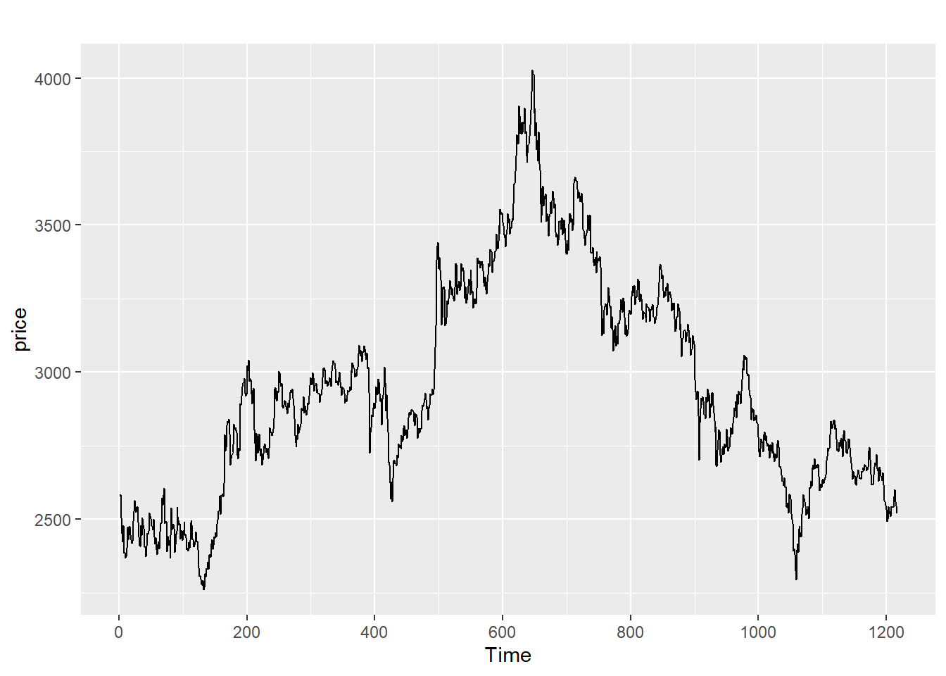
Figure 1: SSE50 index time series plot.

4. Results

4.1. Stationary Test

In order to further confirm the non-stationary of SSE50 index, the ACF test are conducted in this paper, and the results are presented in table 1.

Table 1: Augmented dickey-fuller test.

According to the ADF test findings in Table 1, the time series possesses a unit root, which suggests it is a non-stationary time series. So, it needs to be differenced before modeling and analyzing [8].

4.2. White Noise Test

ACF identifies if there is a correlation between the current stock price and all of the prices from a specific time in the past. PACF describes the correlation between the present price simply and a certain price in the past. Both values range from -1 to 1 [9]. The stronger the correlation, the closer the absolute value is to 1. The linear correlation between the two is lower as the absolute value gets closer to 0 [10].

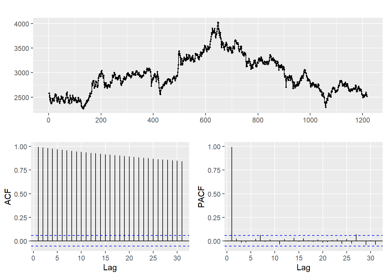
Figure 2: ACF & PACF test.

In figure 2, the blue dotted line represents the error range. When the value does not surpass the blue dotted line, it is essentially assumed that they are not correlated.

This is because the ACF are above the critical value, indicating that this time series is not white noise. This data can be considered to be a non-stationary series when the ACF gradually decrease to 0 and the PACF abruptly drops to 0 after lag1 [11]. Alternately, the p-value is higher than 0.99 according to the ADF test, accepting the null hypothesis that this data is not stationary.

Because the ARIMA model is based on the fact that the data being analyzed must be a stationary time series. The next step involves transforming the non-stationary data into stationary data using differencing. After the transformation, it can be shown from table 2 that ADF test is performed and the p-value is less than 0.01, the null hypothesis is rejected and the data is stationary.

Table 2: Augmented Dickey-Fuller test.

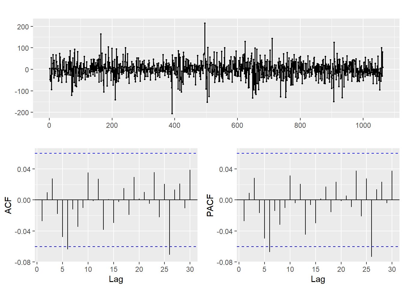
Figure 3: ACF & PACF test after 1 differencing.

The upper part of figure 3 states the new time series data after performing one differencing. It is obvious that it fluctuates up and down around 0. Lag6 and lag26 in the ACF plot exceed the critical values, so the new time series is not white noise.

4.3. Fitting Model

Applying the function auto.arima in the R Studio can determine the parameters in the ARIMA, and the model is tested for residuals. If it passes the Ljung-Box test, it implies that there is no autocorrelation between the residuals and that the model does not require additional correction or adjustment. Table 3 demonstrates that the p-value for the Ljung-Box test is greater than 0.05, indicating that the model passes the residuals test.

Table 3: Ljung-box test.

4.4. Prediction Analysis of the Model

According to figure 4, the ARIMA(0,1,0) model was utilized to predict 152 values (blue line), which was compared to the 152 observations (red line) previously set aside, and the model was found to be statistically soundly fitted.

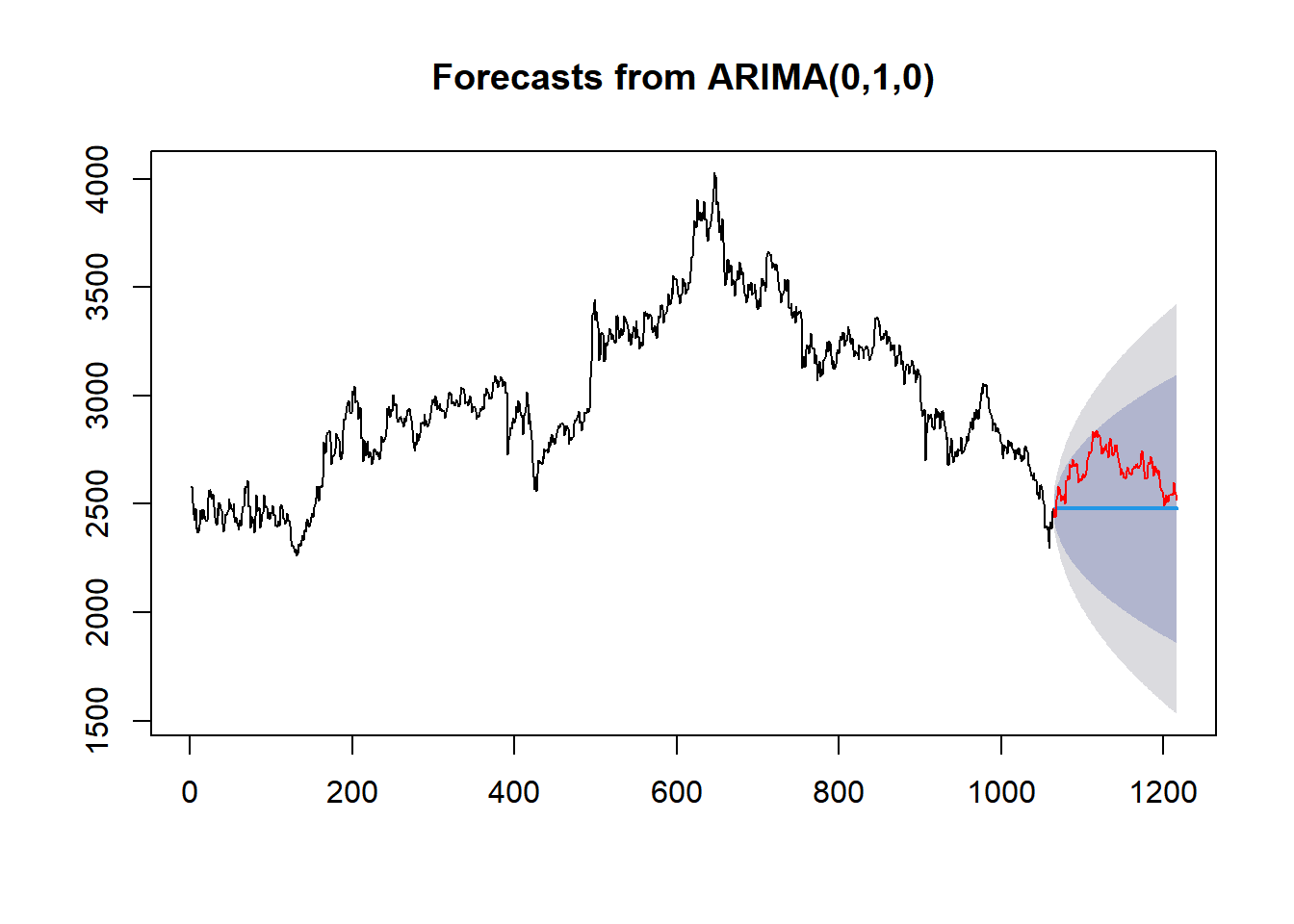
Figure 4: Forecasts from ARIMA(0,1,0).

5. Discussion

With the booming global financial market, more and more investors begin to use mathematical methods to examine stock movements, and make predictions and assessments of stocks from both theoretical analysis and experience, so as to formulate investment strategies [2].

Based on the time series data of SSE50 index selected in this paper, the impact of the daily closing price of the SSE50 index over time is investigated by the empirical method of ARIMA difference integrated moving average autoregressive model fitting, and it is inferred that SSE50 index will fluctuate constantly in the second half of 2023.

Regarding the establishment of the time series model in this paper, on the one hand, because the study has made one difference to the data, there will be some missing information, but it will make the data series more stationary and easier to make predictions, which will lead to better results and help people to make better decisions. On the other hand, stock market investment is closely related to the psychological factors of the investors with great uncertainty, which in turn will have an impact on the prediction.

In many cases, even though the ARIMA model passes the residual test, there is still some information that has not yet been uncovered as can be seen in the ACF plot. And as shown in table 2, the actual p-value is smaller than 0.01, which may cause over fitting and make the results less obvious. Therefore, it is not rigorous to judge the fit of the model just based on the p-value.

Although the ARIMA model successfully predicted the range of SSE50 index during the 152 days of the test set, the index had a U-shaped fluctuation during this period. And the prediction did not reflect the changes and fluctuations of the index, but only reflected a result, which is not a good reference for investors who prefer short-term investment.

In addition, the actual volatility of the stock market is relatively large, subject to the interference of many influencing factors, such as market risk, political risk, technical risk and so on [1]. Simply relying on one model to do the prediction is not enough, and even sometimes with the same indicators of different time periods of data for prediction will lead to different predictions. Therefore, it needs to be combined with other methods and economic facts to make a comprehensive judgment.

6. Conclusion

In this paper, the closing price time series of SSE50 index of Shanghai stock market from June 21, 2018 to June 21, 2023 is taken as the data set. On this basis, an ARIMA(0,1,0) model is constructed for the sample period using the mature time series modeling technique using R Studio to fit and forecast the SSE50 index. The model fitting effect and forecasting accuracy are examined, and the results are well-fitted.

Stock price forecasting is still a difficult topic because of the stock market's volatility, which leaves it full of uncertainty. Nevertheless, because the time series forecasting theory has a positive short-term forecasting impact, it has been acknowledged as an effective method of statistical forecasting of stock price movements. Currently, there are comparatively more techniques available for predicting time series trends, such as gray forecasting, exponential stationary, threshold autoregression, etc. Every technique has some predictive benefits. Due to the fact that each technique is developed to address a particular issue, there are, however, certain drawbacks as well. In this paper, the forecasting technique employed is the ARIMA model, which is comparatively more effective. Comparison of the final forecasts with the actual values revealed that the predictions were more accurate in the near term, showing that the model can produce more accurate results when predicting stocks in the short-term future.

In addition, the stock market's actual volatility is rather high, and it is disturbed by several influencing factors such as market risks, political risks, and technical risks. Simply relying on a single model to do stock price prediction is far from enough. Even sometimes using the same indicator for different time periods of data for prediction will lead to different prediction results. Therefore, stock investment requires a combination of other methods and economic facts to make a comprehensive judgment.

In the next phase of the research, in order to overcome the shortcomings of ARIMA model, which is only accurate in short-term forecasting and unable to predict the fluctuations, we can use LSTM model and BP model to forecast the index and use GARCH model to predict the fluctuations of the index, which can strengthen the corroboration of the results in various aspects.

References

[1]. Zhang, Y., & Sun, Y. (2019). Empirical study on Shanghai Stock Exchange Index Analysis and Prediction based on ARIMA Model. Economic Research Guide, (11), 131-135.
[2]. Xu, S., & Hu, T. (2023). Analysis and Forecast of Shanghai Composite Index Based on Time Series. Economic Research Guide, (07), 88-90.
[3]. Li, H. (2022). Analysis of the Trend of the Shanghai Stock Exchange 50 Index based on the ARIMA-BP-LSTM Model. Shandong University.
[4]. Wang, H., & Lin, J. (2017). Analysis and Forecast of Shanghai Stock Exchange 50 Index Based on ARIMA Model. Times Finance, (24), 143-144.
[5]. Hu, Z., Ma, J., Yang, L., Yao, L., & Pang, M. (2019). Monthly electricity demand forecasting using empirical mode decomposition-based state space model. Energy & Environment, 30(7), 1236–1254.
[6]. Pennekamp, F., Iles, A. C., Garland, J., Brennan, G. et al. (2019). The intrinsic predictability of ecological time series and its potential to guide forecasting. Ecological Monographs, 89(2), 1–17.
[7]. Xu, D., Zhang, Q., Ding, Y., & Huang, H. (2020). Application of a Hybrid ARIMA–SVR Model Based on the SPI for the Forecast of Drought—A Case Study in Henan Province, China. Journal of Applied Meteorology and Climatology, 59(7), 1239–1259.
[8]. Shuai, Y., & Zhou, Z. (2019). GDP Analysis and Comparison in Coastal Cities Based on Time Series Analysis. Journal of Coastal Research, 98(SI), 402-406.
[9]. Huang, S. (2022). Analysis and Forecast of Stock Price Based on ARIMA Model: Taking China Merchants Bank as An Example. Management & Technolosy of SME, (11), 184-187
[10]. Husby, T., & Visser, H. (2021). Short- to medium-run forecasting of mobility with dynamic linear models. Demographic Research, 45, 871–902.
[11]. Xu, S., & Liang, X. (2019). Research on Stock Price Prediction Based on ARIMA-GARCH Model. Journal of Henan Institute of Education (Natural Science Edition), 28(4), 20-24.
Cite this article
Zhou,Y. (2023). Stock Price Forecasting and Analysis Algorithm Based on ARIMA Taking Shanghai Stock Exchange 50 Index as an Example. Advances in Economics, Management and Political Sciences,48,247-255.
Data availability
The datasets used and/or analyzed during the current study will be available from the authors upon reasonable request.
Disclaimer/Publisher's Note
The statements, opinions and data contained in all publications are solely those of the individual author(s) and contributor(s) and not of EWA Publishing and/or the editor(s). EWA Publishing and/or the editor(s) disclaim responsibility for any injury to people or property resulting from any ideas, methods, instructions or products referred to in the content.
About volume
Volume title: Proceedings of the 2nd International Conference on Financial Technology and Business Analysis
© 2024 by the author(s). Licensee EWA Publishing, Oxford, UK. This article is an open access article distributed under the terms and
conditions of the Creative Commons Attribution (CC BY) license. Authors who
publish this series agree to the following terms:
1. Authors retain copyright and grant the series right of first publication with the work simultaneously licensed under a Creative Commons
Attribution License that allows others to share the work with an acknowledgment of the work's authorship and initial publication in this
series.
2. Authors are able to enter into separate, additional contractual arrangements for the non-exclusive distribution of the series's published
version of the work (e.g., post it to an institutional repository or publish it in a book), with an acknowledgment of its initial
publication in this series.
3. Authors are permitted and encouraged to post their work online (e.g., in institutional repositories or on their website) prior to and
during the submission process, as it can lead to productive exchanges, as well as earlier and greater citation of published work (See
Open access policy for details).