1. Introduction

In the decades following Markowitz's introduction of the Mean-Variance model (MV), portfolio theory has been extensively researched and utilized [1]. The concept of investment portfolio is not simply to allocate funds to different assets, but to maximize the expected return under a given risk level through ingenious trade-offs and optimization. The importance of investment portfolio lies in its ability to help investors achieve effective allocation of funds and diversification of risks and improve the overall performance of the investment portfolio.

However, some traditional portfolio methods have certain limitations, such as the assumption of asset returns, simplification of investors' risk attitudes, and the handling of correlations between assets. As time has passed, novel portfolio approaches have surfaced. Certain techniques take into account the nonlinear association between assets and the features of non-normal distribution. Examples of such techniques include the Value at Risk (VaR) model, Conditional Value at Risk (CVaR) model, and Omega model [2-4]. These models provide more choice and flexibility in taking into account investors' different attitudes and preferences for risk [5].

In some portfolio-based studies, many scholars focus on selected stocks. Selecting high-quality stocks for investment portfolios is an important factor in improving portfolio performance [6]. Some studies have screened high-quality stocks through multi-factor performance, that is, comprehensive consideration of stock fundamentals, market value, and technical indicators. Based on this, investment portfolios can effectively increase the rate of return [7-8]. Some studies combine classic portfolio strategies, such as pair trading, by selecting stocks with different trends in the same industry, setting buying and shorting criteria to select stocks to build a portfolio [9-10]. The advantage of this method is that it can use the relative value relationship between stocks to achieve portfolio optimization in different market environments. There are also some studies that combine machine learning algorithms with investment portfolios, first use machine learning algorithms to predict future stock prices and build investment portfolios based on the predicted prices. By analyzing and learning from a vast amount of historical data, these algorithms can improve the accuracy of predicting future market trends. Incorporating these predictions into portfolio optimization can lead to more effective investment decision-making [11-12]. At the same time, the reinforcement learning method also shows potential in the construction of portfolio strategies. Through interactive learning with the environment, the agent can make corresponding trading decisions according to market changes [13].

The research in this paper is to combine the deep learning algorithm (LSTM, GRU, CRNN, TCN) with portfolio construction methods (Mean-Variance, Mean-CVaR) to build the portfolio strategies, then select stocks from different industries in the US stock market, and evaluate the effectiveness of the strategies based on cumulative returns. The innovation of this paper mainly lies in two aspects. One is that CRNN and TCN are rarely used in existing research. This paper combines the prediction advantages of deep learning with portfolio models to provide a variety of ideas for portfolio construction; secondly, existing literature mostly uses Mean-Variance in portfolio construction. This paper also introduces Mean-CVaR model and optimizes the MV model through factor score constraints.

2. Data

In order to better diversify risks and respond to market changes, this paper selects six stocks from different industries such as technology industry, financial industry, medical industry, energy industry, and catering industry in the U.S. stock market: 'AAPL', 'GS', 'JNJ', 'KO', 'XOM', 'MCD'. The stock data comes from Yahoo Finance and is imported through yfinance in python. To validate the strategies’ effectiveness, this research examines stock transactions in two distinct market environments: bull market (2011/01/01—2013/06/30) and bear market (2020/01/01—2022/06/30). The training set comprises the first 80% of the data, while the test set consists of the remaining 20% of the data. This research employs four deep learning algorithms to predict the adjusted close of each stock on the last 20% of trading days. Subsequently, Mean-Variance and Mean-CVaR methods are utilized to construct portfolios. The performance of these strategies is then compared across different real market environments.

The Table 1 below shows that stocks exhibit higher standard deviation during the bear market, indicating that the stock price has higher volatility and may face higher risks. Skewness analysis reveals a leftward skew in the distribution of stock prices during the bear market, indicating a higher proportion of lower values compared to a normal distribution.

Table 1: The summary of data.

3. Models

3.1. Four Deep Learning Algorithms

3.1.1. LSTM

Long Short-Term Memory is a specialized type of Recurrent Neural Network (RNN) that incorporates three distinct gates: forget gate (selectively discards unnecessary historical information), input gate (selectively adds certain historical information to the memory cell), and output gate(selectively passes certain historical information from the memory cell to the output). These gates allow LSTM to choose which historical stock price information to retain or discard over time and update new information. In stock price prediction, LSTM can predict future stock price trends by learning long-term dependencies and important features of historical stock price data.

\( Forget Gate: {f_{t}}=σ({W_{f}}\cdot [{h_{t-1}},{x_{t}}]+{b_{f}}) \) (1)

\( Input Gate: {i_{t}}=σ({W_{i}}\cdot [{h_{t-1}},{x_{t}}]+{b_{i}}) \) (2)

\( Cell State Update: \widetilde{{C_{t}}}=tanh{({W_{C}}\cdot [{h_{t-1}},{x_{t}}]+{b_{C}})} \) (3)

\( New Cell State: {C_{t}}={f_{t}}⊙{C_{t-1}}+{i_{t}}⊙\widetilde{{C_{t}}} \) (4)

\( Output Gate: {o_{t}}=σ({W_{o}}\cdot [{h_{t-1}},{x_{t}}]+{b_{o}}) \) (5)

\( Hidden state: {h_{t}}={o_{t}}⊙tanh{({C_{t}})} \) (6)

\( Output: {y_{t}}=Activation({W_{y}}\cdot {h_{t}}+{b_{y}}) \) (7)

In the equations, the Sigmoid function σ is applied to a linear combination of the previous hidden state ( \( {h_{t-1}} \) ) and the current input ( \( {x_{t}} \) ), with corresponding weight and bias terms ( \( W \) and \( b \) ). The resulting output is then element-wise multiplied (represented by the symbol ⊙) by the output of the hyperbolic tangent function (tanh) applied to another linear combination of the same inputs, with different weight and bias terms. The notation [ \( {h_{t-1}} \) , \( {x_{t}} \) ] indicates that the previous hidden state and current input are concatenated together and treated as a single input.

3.1.2. GRU

Gated Recurrent Unit is a type of neural network that is designed to improve upon traditional recurrent neural networks. It achieves this by introducing two gating mechanisms - the reset gate (selectively forgets outdated and irrelevant stock price information) and the update gate (selectively merges stock price inputs into the current state) - which help the network selectively remember or forget information from previous time steps. In the context of stock price forecasting, GRU has shown promise in accurately predicting future trends by leveraging the long-term dependencies in historical stock price data.

\( Reset Gate: {r_{t}}=σ({W_{r}}\cdot [{h_{t-1}},{x_{t}}]) \) (8)

\( {Update Gate: z_{t}}=σ({W_{z}}\cdot [{h_{t-1}},{x_{t}}]) \) (9)

\( New State: \widetilde{{h_{t}}}=tanh{({W_{h}}\cdot [{r_{t}}⊙{h_{t-1}},{x_{t}}])} \) (10)

\( Hidden state: {h_{t}}=(1-{z_{t}})⊙{h_{t-1}}+{z_{t}}⊙\widetilde{{h_{t}}} \) (11)

\( Output:{ y_{t}}=Activation({W_{y}}\cdot {h_{t}}+{b_{y}}) \) (12)

where \( σ \) represents the Sigmoid function, The element-wise multiplication operation is represented by the symbol \( ⊙ \) , the weight matrix (𝑊) is used to transform the input at each time step, then \( [{h_{t-1}},{x_{t}}] \) includes the previous hidden state ( \( {h_{t-1}} \) ) and the current input ( \( {x_{t}} \) )

3.1.3. CRNN

The core idea of Convolutional Recurrent Neural Network model is to establish a seamless combination between CNN and RNN, so as to simultaneously use CNN to extract local spatial features and RNN to model sequence relationships. This combination enables the CRNN model to efficiently handle sequence data with temporal and spatial correlations.

CNN part:

\( convolutional layer: {c_{i}}=f({W_{i}}*x+{b_{i}}) \) (13)

\( pooling layer(optional): {p_{i}}=Pooling({c_{i}}) \) (14)

RNN part:

\( RNN layer: {h_{t}}=RNN({h_{t-1}},{p_{t}}) \) (15)

\( bidirectional RNN(optional): {h_{t}}=BiRNN({h_{t-1}},{p_{t}}) \) (16)

Fully connected layer and output:

\( fully connected layer: z={W_{o}}*{h_{T}}+{b_{o}} \) (17)

\( output layer: y=Activation(z) \) (18)

This neural network architecture utilizes convolutional layers to generate output maps ( \( {c_{i}} \) ) using activation functions (f) and corresponding weight and bias items ( \( {W_{i}} \) and \( {b_{i}} \) ). These output maps are then processed by pooling layers to produce output features ( \( {p_{i}} \) ). The output from the pooling layer serves as the input for a recurrent neural network (RNN), such as LSTM or GRU, which employs a hidden state ( \( {h_{t}} \) ) to capture temporal dependencies in the input data. The RNN layer's output is further processed by a fully connected layer with weights and biases ( \( {W_{o}} \) and \( {b_{o}} \) ), along with an appropriate activation function (Activation). The final network output is denoted as y.

3.1.4. TCN

Temporal Convolutional Network draws inspiration from convolutional neural networks, and the use of convolutional layers can effectively capture the temporal relationship and local patterns in sequence data, so as to realize the modeling and prediction of sequence data. In stock price forecasting, the TCN model can capture long-term dependencies and local patterns in time series data to help analyze stock price trends and fluctuations.

\( {h_{i}}=g({W_{j}}\cdot x[i:i+k-1]+{b_{j}}) \) (19)

\( {h^{(0)}}=x \) (20)

\( {h^{(l)}}=g({W^{(l)}}\cdot {h^{(l-1)}}+{b^{(l)}})+{h^{(l-1)}} \) (21)

\( {h^{(l)}}=g({W^{(l)}}\cdot {h^{(l-1)}}+{b^{(l)}})+{h^{(l-1)}}+{h^{(0)}} \) (22)

This neural network architecture involves convolutional layers that produce output feature maps ( \( {h_{i}} \) ) using convolutional kernels ( \( {W_{j}} \) represents the weight) applied to subsequences of the input sequence (x[i:i+k-1]). g is nonlinear activation function (such as ReLU), \( {b_{j}} \) is a bias term, the index of the convolutional layer is denoted by l, and \( {h^{(0)}} \) represents the input sequence, ( \( {h^{(l)}} \) ) is used as the output to the next layer.

3.2. Two Portfolio Models

Mean-Variance (MV) and Mean-CVaR (MC) methods share a common objective of balancing risks and returns in investment decision-making, and construct investment portfolios with good risk-return characteristics. For an investment portfolio, its expected return is:

\( E({R_{p}})=\sum _{i=1}^{n}{w_{i}}\cdot {μ_{i}} \) (23)

Subject to

\( \sum _{i=1}^{n}{w_{i}}=1 \) (24)

\( 0≤{w_{i}}≤1 for i=1,2,…,n \) (25)

where the weight assigned to each asset in the portfolio is denoted by \( {w_{i}} \) , and the expected return of each asset is represented by \( {μ_{i}} \)

Mean-Variance model, introduced by Harry Markowitz in the 1950s, aims to identify the optimal portfolio allocation by minimizing the portfolio's variance while maximizing the Sharpe ratio [1]. This approach considers both the expected returns (mean) and the level of risk (variance) associated with each asset in the portfolio. The portfolio variance \( σ_{p}^{2} \) and Sharpe Ratio is:

\( σ_{p}^{2}=\sum _{i=1}^{n}\sum _{j=1}^{n}{W_{i}}\cdot {W_{j}}\cdot {σ_{i}}\cdot {σ_{j}}\cdot {ρ_{ij}} \) (26)

\( Sharpe Ratio=\frac{E({R_{p}})-{R_{f}}}{{σ_{p}}} \) (27)

where \( {ρ_{ij}} \) is the covariance of i and j, and \( {R_{f}} \) is risk free rate.

Mean-CVaR model focuses on the loss exceeding the confidence level and controls the conditional value at risk within a certain level [3].

\( {CVaR_{p}}=\frac{1}{1-α}\int _{0}^{α}{VaR_{p}}(q) dq \) (28)

where \( {CVaR_{p}} \) represents the CVaR of the portfolio, \( α \) is the confidence level, and \( {VaR_{p}}(q) \) represents the VaR of the portfolio at the quantile \( q \) .

4. Results

4.1. Prediction Evaluation

This study evaluates the performance of different models in predicting stock adjusted close by using two commonly metrics - mean squared error (MSE) and mean absolute error (MAE). This part is able to identify which models perform the best in predicting stock adjusted close and provide valuable insights for future research and investment decision-making.

\( MSE=\frac{1}{n}\sum _{t=1}^{n}{({y_{t}}-\hat{{y_{t}}})^{2}} \) (29)

\( MAE=\frac{1}{n}\sum _{t=1}^{n}|{y_{t}}-\hat{{y_{t}}}| \) (30)

The data in Table 2 indicates that CRNN and TCN have lower MSE and MAE compared to LSTM and GRU. Furthermore, the error gap between the models is larger in the bull market forecast, while it is smaller in the bear market forecast. Overall, TCN outperforms other models in stock price prediction, while LSTM exhibits larger prediction errors.

Table 2: The Performance of different models.

4.2. Portfolio Construction

The data predicted by different deep learning models is used to construct the investment portfolio, and the weight distribution of each asset is obtained. After that, the effect of the portfolio is evaluated in the real market environment within the transaction date. This part implements the buy-and-hold strategy, that is, after determining the weight of each stock, hold it until the end of the maturity date, without considering transaction costs, leverage, and short selling.

4.2.1. Bull Market

The cumulative return of the S&P 500 during the specified time period is 1.057. The first sub-graph demonstrates that the cumulative returns of the four deep learning algorithms combined with mean-variance (MV) strategies surpass that of the S&P 500, indicating their ability to outperform the market. Among these strategies, GRU+MV and TCN+MV exhibit higher cumulative returns of 1.1525 and 1.1517, respectively, surpassing the other two strategies. In the second sub-graph, the cumulative return of GRU+MC is comparable to that of the S&P 500, while the TCN+MC strategy performs the best, exhibiting a higher cumulative return of 1.091 compared to the S&P 500. Overall, the sub-graphs illustrate that given a consistent prediction result, the MV strategies demonstrates superior performance compared to the MC strategies (See Figure 1).

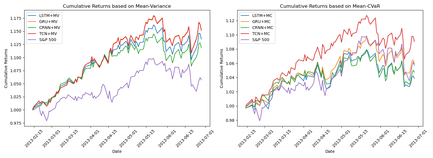
Figure 1: Portfolio performance during bull market.

4.2.2. Bear Market

The cumulative return of S&P 500 over the time period is 0.848. As can be seen from the first sub-graph, the cumulative returns of the four deep learning algorithms combined with MV strategies surpass 1 and significantly outperform the S&P 500. This indicates that these four strategies exhibit market-beating performance and yield higher returns. Numerically, the cumulative returns of the four strategies are relatively close, all around 1.1. In the second sub-graph, the cumulative returns of the four deep learning algorithms combined with MC strategies exceed that of the S&P 500. Among them, the CRNN+MC strategy achieves the highest cumulative return of 1.06. In general, while all the investment strategies produce better cumulative returns than the benchmark index, the strategies based on the MV model achieved the highest returns (See Figure 2).

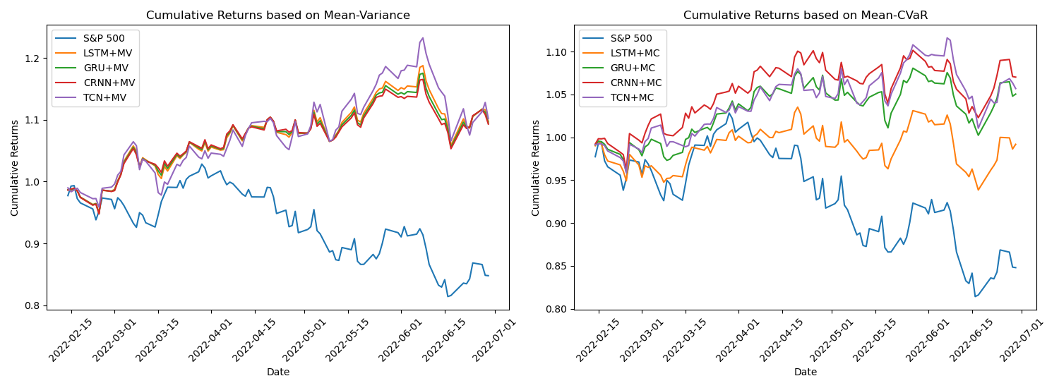
Figure 2: Portfolio performance during bear market.

4.3. Factor Scores

Based on the results, the use of MV in portfolio construction yields better results than MC when prediction outcomes are fixed. This paper extends the combination of four deep learning algorithms with the MV model and introduces score constraints for portfolio optimization. The selected factors include size factor (market capitalization), value factors (PE, PS), volatility factor (stock price volatility), momentum factors (RSI, daily trading volume), and profitability factor (daily returns) [14]. Based on the data collected during the training period, factors that have the highest positive impact on stock returns are assigned a score of 6, while the scores decrease sequentially in descending order. The lowest score assigned is 1. The final score for each stock is calculated as the average score, representing its overall performance.

Let vector s represent the scores of all stocks, and vector w represent the weights assigned to the stocks. The constraint T is introduced to ensure that the portfolio score exceeds the target constraint. The following condition is incorporated into the optimization of the MV model:

\( {w^{T}}\cdot s≥T \) (31)

Different T values will bring different investment returns. In a bull market, lower T score constraints result in higher cumulative returns. When the minimum T is set at 2.5, the cumulative return of the portfolio for the four strategies is 1.1525, higher than that of the S&P 500, 1.0572. In the bear market, all five T value constraints lead to cumulative returns for the investment portfolio that exceed the S&P 500's performance. The higher the constraint on the T value, the greater the cumulative return. Specifically, with a minimum T of 4.5, the portfolio achieves a cumulative return close to 1.13.

In conclusion, incorporating factor score constraints into the deep learning algorithm + MV framework allows for the identification of stocks with higher potential returns, leading to optimized investment portfolios and superior overall returns (See Table 3 and Figure 3).

Table 3: Optimization with integrated factor scores.

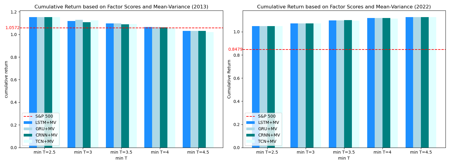
Figure 3: Cumulative returns under factor scores constraints.

5. Conclusion

This article focuses on portfolio construction, combining deep learning algorithms with classic portfolio strategies to construct different portfolio strategies. To assess the effectiveness of the strategy, this paper utilizes market data from both bullish and bearish market conditions, and compares the cumulative return of the portfolio with S&P 500 in a real market environment, and finds that the cumulative returns the strategies combined with the MV are better than those combined with MC. On this basis, this paper selects multiple factors for scoring, and adds factor scores as constraints to the process of portfolio optimization. The results show that the cumulative return has been steadily improved in both bull and bear markets.

This article only considers the investment strategy of buy-and-hold and does not consider the strategy of dynamic weight adjustment as the market changes. At the same time, this article does not consider factors such as transaction costs. These issues are directions for further research.

References

[1]. Markowitz, H. (1952) Portfolio selection. The Journal of Finance, 7, 77–91.
[2]. Alexander, G. J., and Baptista, A. M. (2002) Economic implications of using a mean-VaR model for portfolio selection: A comparison with mean–variance analysis. Journal of Economic Dynamics and Control, 26, 1159–1193.
[3]. Rockafellar, R. T., and Uryasev, S. (2000) Optimization of conditional value-at-risk. Journal of Risk, 2, 21–42.
[4]. Kapsos, M., Christofides, N., and Rustem, B. (2014). Worst-case robust Omega ratio. European Journal of Operational Research, 234, 499–507.
[5]. Xu, W.J., Huang, J.L., Fu, Z. N., and Zhang, W. G. (2022) Research on Black-Litterman portfolio model based on financial text sentiment mining—Evidence from the posting text of eastmoney stock forum and the A share market. Operations Research Transactions, (04),1-14.
[6]. Wang, W., Li, W., Zhang, N., and Liu, K. C. (2020) Portfolio formation with preselection using deep learning from long-term financial data. Expert Systems with Applications, 143, 113042.
[7]. Li, R.Y., and Ye, Z.Q. (2023) Prediction of Fund Returns Based on Machine Learning. Statistics & Decision (11),156-161.
[8]. Bessler, W., Taushanov, G., and Wolff, D. (2021) Factor investing and asset allocation strategies: a comparison of factor versus sector optimization. Journal of Asset Management, 22(6), 488–506.
[9]. Luo, J., Lin, Y., and Wang, S. (2022) Intraday high-frequency pairs trading strategies for energy futures: evidence from China. Applied Economics, 1-15.
[10]. Du, J. (2022) Mean–variance portfolio optimization with deep learning based-forecasts for cointegrated stocks. Expert Systems with Applications, 201, 117005.
[11]. Ma, Y. L., Han, R. Z., and Wang, W. Z. (2020) Prediction-based portfolio optimization models using deep neural networks. IEEE Access, 8, 115393-115405.
[12]. Zhang, N., Yan, S.B., and Fan, D. (2022) Yield Prediction and Portfolio Model Based on Deep Learning. Statistics & Decision, (23),48-51.
[13]. Mang, J., Xie, L., and Xu, H. J. (2023) Integrated deep reinforcement learning portfolio model. Journal of Computer Applications.
[14]. Xie, H. L. and Hu, D. (2017) The Application of Multi-factor Quantization Model in Portfolio: The Comparative Research on LASSO and Elastic Net. Journal of Statistics and Information (10),36-42.
Cite this article
Piao,J. (2023). Portfolio Optimization Based on Deep Learning and Factor Constraints. Advances in Economics, Management and Political Sciences,48,264-273.
Data availability
The datasets used and/or analyzed during the current study will be available from the authors upon reasonable request.
Disclaimer/Publisher's Note
The statements, opinions and data contained in all publications are solely those of the individual author(s) and contributor(s) and not of EWA Publishing and/or the editor(s). EWA Publishing and/or the editor(s) disclaim responsibility for any injury to people or property resulting from any ideas, methods, instructions or products referred to in the content.
About volume
Volume title: Proceedings of the 2nd International Conference on Financial Technology and Business Analysis
© 2024 by the author(s). Licensee EWA Publishing, Oxford, UK. This article is an open access article distributed under the terms and
conditions of the Creative Commons Attribution (CC BY) license. Authors who
publish this series agree to the following terms:
1. Authors retain copyright and grant the series right of first publication with the work simultaneously licensed under a Creative Commons
Attribution License that allows others to share the work with an acknowledgment of the work's authorship and initial publication in this
series.
2. Authors are able to enter into separate, additional contractual arrangements for the non-exclusive distribution of the series's published
version of the work (e.g., post it to an institutional repository or publish it in a book), with an acknowledgment of its initial
publication in this series.
3. Authors are permitted and encouraged to post their work online (e.g., in institutional repositories or on their website) prior to and
during the submission process, as it can lead to productive exchanges, as well as earlier and greater citation of published work (See
Open access policy for details).