1. Introduction

Operational research is a multidisciplinary research field. It solves complex decision-making problems in various fields by designing corresponding mathematical formulas for problems and using the concept of formulas to build virtual models to optimize and analyze the development and optimal solutions of problems. This paper delves into the principles of dynamic programming and explores its application in the field of operations research, particularly in the areas of inventory control and logistics. Dynamic programming was proposed by American mathematician R.E. Bellman in the 1950s. Its basic principle is the optimization principle proposed by Bellman in the book "Dynamic Programming" [1], that is, the optimal decision-making process of multiple stages. As mentioned in the article "A review of approximate dynamic programming applications within military operations research" [2], Dynamic Programming is based on two fundamental principles: optimal substructure and overlapping subproblems [3]. Given a problem and splits the problem into sub-problems until the sub-problems can be solved directly. After getting the sub-question answer, store the answer in memory to reduce double counting. It is a method to obtain the solution of the original problem based on the reverse deduction of the answers to the sub-problems. Generally, these sub-problems are very similar and can be recursively derived through functional relations.

Dynamic programming is committed to solving each sub-problem once and reducing repeated calculations. For example, the Fibonacci sequence can be considered an entry-level classic dynamic programming problem. By solving these subproblems iteratively and combining their solutions, dynamic programming enables the determination of an optimal sequence of decisions, commonly referred to as a decision chain. Dynamic programming utilizes the Markov property to represent decision problems as Markov decision processes, enabling the computation of optimal policies. It leverages self-similarity and sub-problem overlap to avoid redundant computations and improve computational efficiency. However, dynamic programming faces challenges with high-dimensional decision spaces, known as the curse of dimensionality. To overcome this, approximate dynamic programming methods like reinforcement learning algorithms approximate the optimal value function or policy. Dynamic programming finds applications in operations research, solving problems such as dynamic inventory control and the shortest path problem in logistics. While dynamic programming offers powerful modeling capabilities, its computational complexity increases with problem size and dimensionality. Algorithmic design and efficient solution approaches are crucial to address these limitations. The emergence of data-driven approximate dynamic programming, particularly reinforcement learning, presents new opportunities to tackle these challenges and unleash the full potential of dynamic programming as a general-purpose modeling tool.

2. Application Scenarios of Dynamic Programming

The first is the optimal solution problem. The main purpose of the optimal solution problem is to find the largest subarray, the longest increasing subarray, the longest increasing subsequence, or the longest common substring, subsequence, etc.; there are also the famous knapsack problem and the most reasonable use of coupons. The second is the feasibility analysis of the problem. This includes finding whether a path with a sum of x can be realized or finding a feasible path that meets certain conditions, such as constraints, or the probability of occurrence of a certain event. Such problems can be summarized as feasibility problems and solved using dynamic programming. Finally, in addition to finding the maximum value and feasibility, finding the total number of solutions is also a relatively common type of dynamic programming problem. This type of problem will give a data structure and limiting conditions, so as to calculate all possible paths of a plan, then this kind of problem belongs to the problem of finding the total number of plans.

3. Multi-Stage Decision-Making in Dynamic Programming

3.1. The Process of Decision-Making

The decision of the current stage will often affect the decision of the next stage, and the decisions of each stage constitute a decision, a sequence called a strategy. There are several decisions to choose from in each stage, so there are many strategies to choose from. How to choose an optimal strategy among these strategies is a multi-stage decision-making problem. Generally, it starts from the initial state and reaches the end state by selecting intermediate-stage decisions. These decisions form a sequence of decisions and at the same time determine a course of action (usually an optimal course of action) to complete the entire process. Each decision stage produces a set of states, and finally, the optimal solution is obtained through a set of decision sequences. Problems using dynamic programming must satisfy the optimization principle and have no after-effects. According to the book “Introduction to Probability Models - Operations Research: Volume Two” [4], Many applications of dynamic programming reduce to finding the shortest (or largest) path that joins two points in a given network.

In any decision analytics problem, the final goal should be to find the best way to make some set of decisions. If there’s more than one decision, the problem should be divided into stages, represented by k. Divide the given problem-solving process into several interconnected stages appropriately to solve the problem. The number of stages may be different if the process is different. A stage variable is continuous if the process can make a decision at any time and an infinite number of decisions are allowed between two different times. When solving such multi-stage problems, it is first necessary to divide the problem into several stages according to the time or space characteristics of the problem. When dividing the stages, note that the divided stages must be ordered or sortable, otherwise, the problem cannot be solved. Then the various objective situations in which the problem develops at each stage are expressed in different states. In this process, the choice of state must satisfy the non-consequence effect. Write the state transition equations after determining the decision. Since there is a natural connection between decision-making and state transition, the state transition is to derive the state of this stage based on the state and decision-making of the previous stage. After obtaining the state transition equation, this recursive equation requires a recursive termination condition or boundary condition. In each stage k, the state, represented by xk, consists of all the information about the decisions at earlier stages that can have any bearing on the decision at this stage and later ones. The state represents the natural state or objective condition faced at each stage, which does not depend on people's subjective will, and is also called an uncontrollable factor. Within each stage k, each state xk has a value. For a state xk in stage k, its value is written Vk (xk). This value is the best profit (or lowest cost) that you can obtain from stage t to the end, given that you are in state xk at stage k. After the state of a stage is given, a choice (behavior) that evolves from this state to a certain state in the next stage is called decision-making. Since the state satisfies no aftereffect, only the current state is considered when choosing a decision at each stage without considering the history of the process. As shown in Figure 1, given the value of the state variable x(k) in the k stage, if the decision variable in this stage is determined, the state variable x(k+1) in the k+1 stage is also completely determined, that is The value of x(k+1) changes with the value of x(k) and the decision u(k) of the k-th stage, then this relationship can be regarded as (x(k), u(k)) and x The corresponding relationship determined by (k+1) is represented by x(k+1)=Tk(x(k),u(k)).

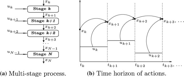
Figure 1: Multi-stage decision process [5].

This is the law of state transition from stage k to stage k+1, called the state transition equation. This process makes dynamic programming possible to compute the value of every state by working backwards from the last stage.

3.2. Markov Property

No after-effect is also called Markov property. The article "Markov Decision Processes" [6] simply describes Markovianness as "In the general theory a system is given which can be controlled by sequential decisions. The state transitions are random and we assume that the system state process is Markovian which means that previous states have no influence on future states". In the real world, many processes can be reduced to Markov processes, such as Brownian motion - the random motion of tiny particles or particles in a fluid. When we buy low-value items, it is usually a Markov process. For example, when looking at the dazzling milk in front of the supermarket shelves, when considering which brand of milk to choose, there are usually two factors that have the greatest impact on people: which brand did you buy last time and what brand are you currently using? And now which milk brand in the supermarket has the most promotion? To sum up: the Markov process is that the future state has nothing to do with other historical states, but only with the current state.

3.3. Self-Similarity

If the optimal solution to a problem includes the optimal solution to the same problem on a smaller scale, then dynamic programming can be used to solve it. The self-similarity of dynamic programming is the basis for stage division, and each stage or subsequent sub-process has a similarity with the whole, which is essentially the basis for the divisibility of dynamic programming problems and the solution of detachable sub-processes.

3.4. Overlap of Sub-Problems

Dynamic programming improves the original search algorithm with exponential time complexity into an algorithm with polynomial time complexity. The key is to solve the redundancy, which is the fundamental purpose of the dynamic programming algorithm [7]. That is, the sub-problems are not independent, and a sub-problem may be used multiple times in the next stage of decision-making. (This property is not a necessary condition for the application of dynamic programming, but without this property, the dynamic programming algorithm has no advantage over other algorithms). Dynamic programming is essentially a technique of exchanging space for time. During its implementation, it has to store various states in the generation process, so its space complexity is greater than other algorithms. For a deterministic decision process, the state of the next segment in the problem is fully determined by the state and decision of the current segment. The stochastic decision-making process, the difference between it and the deterministic decision-making process is that the state of the next stage cannot be completely determined by the state and decision of the current stage, but the state of the next stage is determined according to a certain probability distribution. This probability distribution is fully determined by the state and policy of the current segment.

4. Applications of Dynamic Programming in Operations Research

Dynamic programming finds numerous applications in Operations Research across various domains. One such area is Inventory Management, where dynamic programming techniques assist in identifying optimal inventory replenishment policies by considering factors such as demand variability, holding costs, and ordering costs [8]. Resource Allocation is another field where dynamic programming plays a crucial role in optimizing the allocation of limited resources, such as personnel, equipment, or funds, to maximize system performance or minimize costs [9]. In Project Scheduling, dynamic programming enables efficient scheduling of complex projects by taking into account dependencies, resource constraints, and time-related objectives. Routing and Network Optimization benefit from dynamic programming algorithms that can determine optimal routes in transportation networks, minimizing costs or travel time [10]. Lastly, in Production Planning, dynamic programming techniques optimize production planning decisions, including batch scheduling, machine assignment, and job sequencing, to enhance productivity and minimize costs.

5. Advantages and Limitations of Dynamic Programming

Dynamic programming has several advantages that make it a valuable approach to problem-solving. Firstly, it guarantees the attainment of optimal solutions by leveraging optimal substructure. This means that it can identify the globally best solutions for problems. Secondly, dynamic programming enables efficient computation by reusing previously computed results through memoization. This technique significantly reduces computational effort, especially for problems with overlapping subproblems. Thirdly, dynamic programming exhibits versatility, as it can be applied to a wide range of problems across different domains, making it a flexible tool within operations research.

Despite its advantages, dynamic programming does have limitations that should be considered. One limitation is the curse of dimensionality, first introduced by Bellman [1], where the computational complexity of dynamic programming algorithms increases exponentially with the size of the problem. As shown in Figure 2, the problem of data sparsity is caused by high dimensionality: Suppose there is a feature whose value range d is evenly distributed between 0 and 2, and its value is unique for any point. In the one-dimensional picture displayed in Figure 2a, all points are in the same dimension and are relatively closely related to each other. Figure 2b shows that these points in the two-dimensional space are re-divided due to the addition of a new dimension, and the points that were originally determined to belong to the same zone space may not belong to the same space at this time. The green point that was in a 1D unit-sized container is now no longer inside that 2D square. Figure 2c illustrates objects in a 3D feature space. When the dimension is close to a certain level, to obtain the same number of training samples, it is necessary to obtain a value range close to 100% in almost every dimension or to increase the total sample size, but the sample size is always limited. Due to the curse of dimensionality, the points become sparser by adding more dimensions.

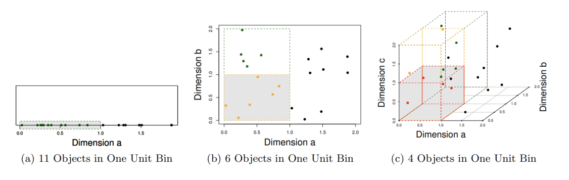
Figure 2: The curse of dimensionality (a) 11 objects in one unit bin (b) 6 objects in one unit bin (c) 4 objects in one unit bin (see online version for colours) [11].

This restricts the scalability of dynamic programming for solving large-scale problems efficiently. Another limitation is that dynamic programming is most effective for problems with discrete decision spaces, and its application to continuous or mixed-integer problems is limited. Finally, dynamic programming may require substantial memory resources to maintain a dynamic programming table or memoization array. Consequently, the memory requirements can impose restrictions on the size of problems that can be effectively solved using dynamic programming techniques. When the system model is Markovian and the objective function is separable and nested monotonic, based on the optimality principle proposed by Bellman, dynamic programming can be used to decompose the multi-stage global optimal decision-making problem into a series of local optimization problems on segments. Compared with other solutions, especially in the presence of disturbances or in stochastic situations, dynamic programming can always effectively provide an optimal feedback control strategy under the current information set. However, no breakthrough has been made in overcoming the Achilles' heel of dynamic programming, which Bellman calls the "curse of dimensionality". Therefore, it is urgent to seek an effective algorithm to overcome the curse of dimensionality for the application of dynamic programming in high-dimensional problems. In addition, the optimal strategy obtained by solving an inseparable optimization problem does not satisfy the principle of optimality or does not have time consistency, which involves the rationality of the inseparable optimization problem model itself, so how to find a set of separable optimization problems to approximate A given inseparable optimization problem also has its obvious importance for the development of dynamic programming.

6. Conclusion

Dynamic programming is a very powerful modeling tool. Basically, if a multi-stage decision problem cannot be written as a dynamic programming model, it is likely that the optimal solution to the problem is also difficult to find. For example, in the field of operations management, the so-called dynamic inventory control problem is a very classic dynamic programming problem. In the field of logistics and transportation, the shortest path problem, one of the core problems, is also a classic dynamic programming problem. In fact, any Markov decision process problem with a finite state space can be written as a shortest path problem. The price of powerful modeling capabilities is that it is often easy for people to write all kinds of dazzling dynamic programming recursions, but it may take a long time to find an "efficient" algorithm to solve them. This is because dynamic programming is a mathematical programming modeling idea, especially when the dimension of the decision space is large, the dynamic programming algorithm will suffer from the famous curse of dimensionality, that is, the algorithm solution time increases exponentially with the problem scale. Therefore, in order to really solve complex dynamic programming problems, people can only approximate the solution, which is also called approximate dynamic programming. In recent years, with the upsurge of machine learning, data-driven approximate dynamic programming has gradually become familiar again, especially one type of approximate algorithm, the so-called reinforcement learning algorithm. In conclusion, dynamic programming has existed as a research field for more than half a century. At present, it has received another wave of attention, and its research difficulty lies in the design and solution of algorithms for high-dimensional problems as a general-purpose modeling tool.

References

[1]. Bellman, R.E. (1957) Dynamic Programming. Princeton University Press, Princeton.
[2]. Rempel, M., and J. Cai. “A Review of Approximate Dynamic Programming Applications within Military Operations Research.” Operations Research Perspectives, vol. 8, 2021, p. 100204, https://doi.org/10.1016/j.orp.2021.100204.
[3]. de Souza, E. A., Nagano, M. S., & Rolim, G. A. (2022). Dynamic programming algorithms and their applications in Machine Scheduling: A Review. Expert Systems with Applications, 190, 116180. https://doi.org/10.1016/j.eswa.2021.116180
[4]. Winston, Wayne L. Introduction to Probability Models, Operations Research: Volume Two. Thomson Learning, 2004.
[5]. Faísca, Nuno P., et al. “A Multi-Parametric Programming Approach for Constrained Dynamic Programming Problems.” Optimization Letters, vol. 2, no. 2, 2007, pp. 267–280, https://doi.org/10.1007/s11590-007-0056-3.
[6]. Bäuerle, Nicole, and Ulrich Rieder. “Markov Decision Processes.” Jahresbericht Der Deutschen Mathematiker-Vereinigung, vol. 112, no. 4, 2010, pp. 217–243, https://doi.org/10.1365/s13291-010-0007-2.
[7]. Ferrentino, E., & Chiacchio, P. (2018). A topological approach to globally-optimal redundancy resolution with Dynamic Programming. ROMANS 22 – Robot Design, Dynamics and Control, 77–85. https://doi.org/10.1007/978-3-319-78963-7_11
[8]. Silver, E. A. (1981). Operations research in inventory management: A review and Critique. Operations Research, 29(4), 628–645. https://doi.org/10.1287/opre.29.4.628
[9]. Mohammad Hossein Bateni, Yiwei Chen, Dragos Florin Ciocan, Vahab Mirrokni (2021) Fair Resource Allocation in a Volatile Marketplace. Operations Research 70(1):288-308.
[10]. Şeref, O., Ahuja, R. K., & Orlin, J. B. (2009). Incremental network optimization: Theory and Algorithms. Operations Research, 57(3), 586–594. https://doi.org/10.1287/opre.1080.0607
[11]. Rajput, D. S., Singh, P. K., & Bhattacharya, M. (2012). Iqram: A high dimensional data clustering technique. International Journal of Knowledge Engineering and Data Mining, 2(2/3), 117. https://doi.org/10.1504/ijkedm.2012.051237
Cite this article
Yi,R. (2023). Optimizing Operations Management and Business Analytics Strategies under Uncertainty: Dynamic Programming. Advances in Economics, Management and Political Sciences,49,150-156.
Data availability
The datasets used and/or analyzed during the current study will be available from the authors upon reasonable request.
Disclaimer/Publisher's Note
The statements, opinions and data contained in all publications are solely those of the individual author(s) and contributor(s) and not of EWA Publishing and/or the editor(s). EWA Publishing and/or the editor(s) disclaim responsibility for any injury to people or property resulting from any ideas, methods, instructions or products referred to in the content.
About volume
Volume title: Proceedings of the 2nd International Conference on Financial Technology and Business Analysis
© 2024 by the author(s). Licensee EWA Publishing, Oxford, UK. This article is an open access article distributed under the terms and
conditions of the Creative Commons Attribution (CC BY) license. Authors who
publish this series agree to the following terms:
1. Authors retain copyright and grant the series right of first publication with the work simultaneously licensed under a Creative Commons
Attribution License that allows others to share the work with an acknowledgment of the work's authorship and initial publication in this
series.
2. Authors are able to enter into separate, additional contractual arrangements for the non-exclusive distribution of the series's published
version of the work (e.g., post it to an institutional repository or publish it in a book), with an acknowledgment of its initial
publication in this series.
3. Authors are permitted and encouraged to post their work online (e.g., in institutional repositories or on their website) prior to and
during the submission process, as it can lead to productive exchanges, as well as earlier and greater citation of published work (See
Open access policy for details).