1. Introduction

Nowadays, constructing an effective investment portfolio is becoming more and more important for investors as market moves quickly. The portfolio optimization is vital to investors determine portfolio strategies [1]. A good investment portfolio can always help investors spread their risk across stocks, bonds, and other types of securities and financial instruments. By investing into a portfolio, investors can bear less volatilities than putting all their funds into an individual security. However, while lowering the risks, investors would like to see a higher return for their portfolios [2]. That is why investors and economist are keen on finding different types of investment strategies and use model to optimize their investment portfolio [3].

There are plenty of models and research on finding optimal investment portfolio at present. One of these is CAPM, the capital asset pricing model, it is very useful in evaluate the investment portfolio and widely used. However, it has problems on the assumptions of the model for example, investors only focus on one period risk and return of portfolio [4]. Sharpe index model, which is a better model than CAPM and gives the accurate weights of each asset in investment, it also measures the risk and return of stocks. Sharpe index model can help to cover the loss of return of securities from other assets in the portfolio [5]. Another is Markowitz model; Markowitz is one of the important models for optimize the investment portfolios by maximize the portfolio return through risk minimized by diversification. But the variance that used for Markowitz model is not totally the risk that taken by the investors [6]. Mean variance model is based on the risk that investors are willing to take, and it encourages risk diversification. However, the potential distribution of returns is not well understood, and no higher level of information is utilized beyond means [7].

All of these models may help to optimize investment portfolio and have their own certain limitation. However, using particular strategies to find investment portfolio and compare them to the performance of the whole market are still lacking. Therefore, the aim of this study is going to compare the performance of different investment portfolios to the market.

2. Data

All the data in this study are from Alpaca (https://alpaca.markets/) and yahoo finance (https://finance.yahoo.com/). To begin with, this paper will choose 5 companies included in New York Stock Exchange, which are Deutsche Bank (DB), Analog Devices (ADI), Johnson & Johnson (JNJ), Beauty Health (SKIN), General Motors Company (GM). This paper Collect the Close pricing data between 2023/01/01 and 2023/04/12 of these companies and is total 100 days. For this study, these data will be split into two parts. The date for the first part is between 2023/01/01 and 2023/03/12, which is 70 days, and the data between this period will be used for finding the Maximum Sharpe ratio portfolio and the Minimum Variance portfolio, and the returns and companies’ weights of them (See Table 1, Figure 1 and Figure 2). Second, the data from 2023/03/12 to 2023/04/12 and use two set of weights have found in first 70 days, will be applied to comprise with S&P 500 index.

Table1: The basic statistics information of these companies.

As the data in Table 1, SKIN has the highest Mean, and the lowest mean is DB. For Variance SKIN is the highest one, JNJ has the lowest variance. Also, SKIN is still the highest in maximum return, and same JNJ is the lowest. However, SKIN has the lowest minimum return, GM is the highest one. After finish construct the table there is a graph of cumulative return for companies with first 70 days.

From the graph that has plotted, that SKIN has the highest cumulative return over this period, and JNJ has the lowest cumulative return of all.

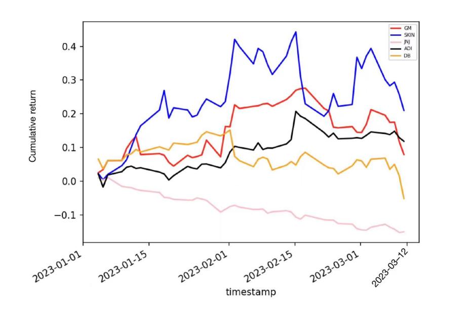
Figure 1: Cumulative return for each ticker in first 70 days.

The reason to choose these five companies is because they are all from different business, and by finding the correlation of them, it shows that they do not have a relative high correlation, which means these assets have not behave in the similar way and choose various assets with low or weak correlation it always can help to reduce the risk of portfolios.

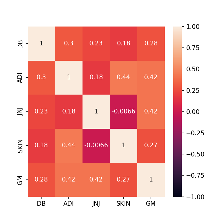
Figure 2: The correlation of five companies.

3. Methods

3.1. Monte Carlo Simulation

The study is going to use Monte Carlo simulation. Monte Carlo simulation is a type of simulation that relies on repeated random sampling and statistical analysis to compute the results [8]. The simulation it is widely used in solving complex problems and optimizing the problems, and with a large number of repeated samplings, it can bring a best result for certain research.

3.2. Expected Weighted Return

By finding the weighted return, this can help us maximize the return of our portfolio, and weighted returns can be calculated as:

\( Weighted return of company= {W_{i}}×{R_{i}} \) (1)

\( Weighted return of portfolio= \sum _{i=1}^{n}{W_{i}}×{R_{i}} \) (2)

\( {W_{i}} \) is the weight of the \( {i_{th}} \) ticker within the whole portfolio.

\( {R_{i}} \) is the return of \( {i_{th}} \) security.

3.3. Portfolio Variance

The variance tells us the how much risk of specific portfolio, and variance is the square of the standard deviation [9].

\( portfolio Variance={{( W_{1 }})^{2}}{( {σ_{1}})^{2}}+{{( W_{2}})^{2}}{( {σ_{2}})^{2}}+2{W_{1 }}×{W_{2}}×{Cov_{1,2}} \) (3)

\( portfolio Standard deviation=\sqrt[]{{{( W_{1 }})^{2}}{( {σ_{1}})^{2}}+{{( W_{2}})^{2}}{( {σ_{2}})^{2}}+2{W_{1 }}×{W_{2}}×{Cov_{1,2}}} \) (4)

\( {W_{i}} \) = the weight of the \( {i_{th}} \) assets

\( {{( σ_{i}} )^{2}} \) = the variance of the \( {i_{th}} \) asset

\( {Cov_{1,2}} \) = the covariance between assets 1 and 2

3.4. Sharpe Ratio

Sharpe ratio shows the relationship between risk and return and considered to be the evaluation of portfolio performance [10].

\( Sharpe ratio= \frac{{R_{i}}-{R_{f}}}{{σ_{i}}} \) (5)

\( {R_{i}} \) is the return of the portfolio.

\( {R_{f}} \) is the risk-free rate of the portfolio.

\( {σ_{i}} \) is the standard deviation of the portfolio.

For this study, assume that the risk-free rate is 0 for every portfolio, which means the value of \( {R_{f}} \) is 0 at this equation. So, with a higher Sharpe ratio, it means how much excess return under each unit of risk of portfolio. When Sharpe ratio is bigger than 1, it always tells us it has a higher return from the investment of the portfolio.

4. Results

For this paper. First, Monte Carlo simulation would randomly generate the weights of companies 10000 times, producing 10,000 sets of weights of the companies included in the portfolio. Thus, returns and volatilities of the portfolios be calculated. Then, an efficient frontier can be constructed and plotted (See Figure 3).

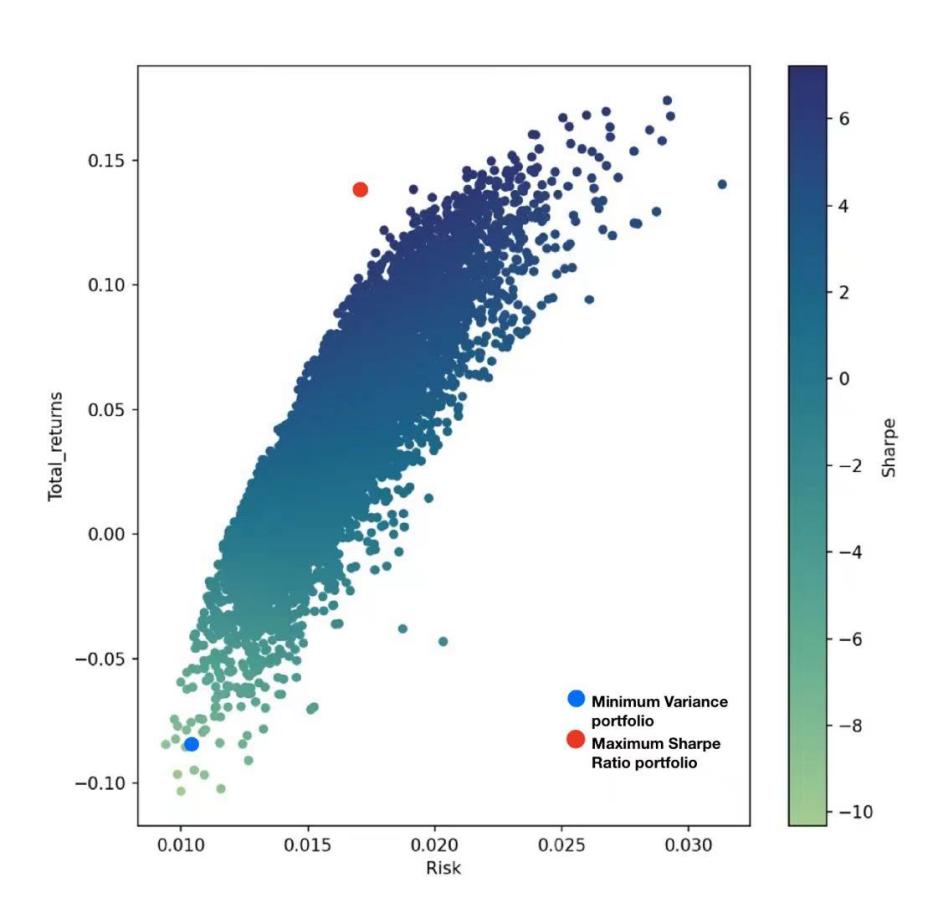
Figure 3: Efficient frontier by simulation.

As seek out which weights perform best. According to the chart and the definition of Variance and Sharpe ratio. This paper will find the weights of Maximum Sharpe ratio portfolio and Minimum Variance portfolio. From these two portfolios, it shows the highest excess return per unit risk, and the excess return with lowest risk, also these two portfolios on the above the graph, which plotted as stars. The set of weights and the weighted returns of portfolio as shown in the Table 2 and Table 3:

Table 2: The weights of companies.

Table 3: The specific data of portfolio between 2023/01/01 and 2023/03/12.

From the Table 2. In Maximum Sharpe ratio, ADI has the biggest weight 73.2%, and JNJ has the lowest weight only 0.375%. For Minimum Variance portfolio, JNJ now has the largest weight 72.47%, and GM becomes to the least weight 2.23%. So, there is a huge difference on weights between these two portfolios. Then this paper constructs another Table 3 which shows the Returns, Volatility and Sharpe ratio between 2023/01/01 and 2023/03/12. From that table. The maximum Sharpe ratio portfolio has the highest Sharpe ratio and a higher return, but it has the maximum Volatility. The Minimum Variance it has the least risk, but the return of this portfolio is negative and has a huge negative value of Sharpe ratio.

Moreover, this paper will continue on testing these two portfolios with the corresponding weights that we have already calculated out in first 70 days, which between 2023/03/12 and 2023/04/12. Also, the study will collect the data of returns of S&P500 in this period and make a comparison, S&P 500 is an index indicate 500 of largest companies of stock exchange in United states, which can be basically represent the whole market.

The graph below shows, the cumulative return of Maximum Sharpe Ratio is 8.02% and the S&P 500 is 6.1%, which means the Maximum Sharpe Ratio portfolio is performed better than the S&P 500. The cumulative return of minimum Variance portfolio is 5.44%, and compared to the S&P 500 6.1%, is performed worse than S&P 500 (See Figure 4).

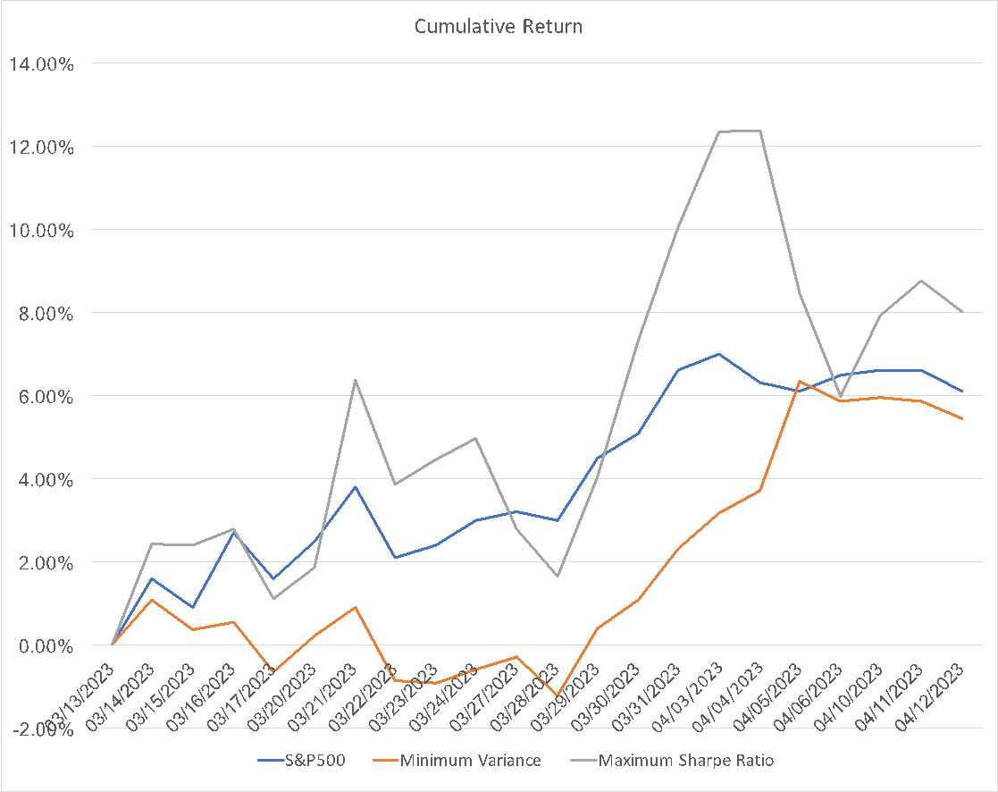
Figure 4: Cumulative return graph of two portfolios and S&P 500.

5. Conclusion

In conclusion, this study constructs an Efficient Frontier by Monte Carlo simulation and make a comparison of Maximum Sharpe Ratio portfolio and Minimum Variance portfolio between the performance of the market. The results demonstrate that, Maximum Sharpe Ratio performed better than S&P 500, Minimum Variance portfolio has a weaker performance than S&P 500. The results of this study can help investors to decide which portfolio to use by comparing the performance with the market and according to the risk preference of investors.

To sum up, the Efficient Frontier approach can optimize the portfolios well, and help to maximize the return or minimize the risk. The Maximum Sharpe Ratio portfolio has a higher cumulative return but with a higher risk, Minimum Variance portfolio has a low risk however the return is low. As these two portfolios seem to be the optimal portfolio, there is no specific answer for which portfolio is better, it is all depend on investor own risk preference. Also, Monte Carlo simulation have some limitations, when simulation is used in portfolio management, itself is based on assumptions which assume there is a perfectly efficient market, so it may not be performed well within the real market. In this case, the simulation may be improved and expanded in the future.

References

[1]. Ivanova, M., and Dospatliev, L. (2017) Application of Markowitz portfolio optimization on Bulgarian stock market from 2013 to 2016. International Journal of Pure and Applied Mathematics, 117(2), 291-307.
[2]. Kresta, A., and Slova, K. (2011) Solving cardinality constrained portfolio optimization problem by binary particle swarm optimization algorithm. Department of Mathematical Methods in Economics, Faculty of Economics, VŠB-Technical University of Ostrava, Sokolská třída, 33(701), 21.
[3]. Zanjirdar, M. (2020) Overview of portfolio optimization models. Advances in mathematical finance and applications, 5(4), 419-435.
[4]. Elbannan, M. A. (2015) The capital asset pricing model: an overview of the theory. International Journal of Economics and Finance, 7(1), 216-228.
[5]. Shah, C. A. (2015) Construction of optimal portfolio using sharpe index model & camp for bse top 15 securities. International Journal of Research and Analytical Reviews, 2(2), 168-178.
[6]. Marling, H., & Emanuelsson, S. (2012) The Markowitz portfolio theory. Journal of Financial Risk Management, 8(2), 1-6.
[7]. Wang, J. (2000) Mean-variance-VaR based portfolio optimization. Valdosta State University.
[8]. Harrison, R. L. (2010) Introduction to monte carlo simulation. In AIP conference proceedings, 1204(1), 17-21
[9]. Chaweewanchon, A., and Chaysiri, R. (2022) Markowitz Mean-Variance Portfolio Optimization with Predictive Stock Selection Using Machine Learning. International Journal of Financial Studies, 10(3), 64.
[10]. Kuo, R.J., and Hong, C.W. (2013) Integration of Genetic Algorithm and Particle Swarm Optimization for Investment Portfolio Optimization. Applied Mathematics & Information Sciences, 7, 2397-2408.
Cite this article
Li,A. (2023). Portfolio Optimization by Monte Carlo Simulation. Advances in Economics, Management and Political Sciences,50,133-138.
Data availability
The datasets used and/or analyzed during the current study will be available from the authors upon reasonable request.
Disclaimer/Publisher's Note
The statements, opinions and data contained in all publications are solely those of the individual author(s) and contributor(s) and not of EWA Publishing and/or the editor(s). EWA Publishing and/or the editor(s) disclaim responsibility for any injury to people or property resulting from any ideas, methods, instructions or products referred to in the content.
About volume
Volume title: Proceedings of the 2nd International Conference on Financial Technology and Business Analysis
© 2024 by the author(s). Licensee EWA Publishing, Oxford, UK. This article is an open access article distributed under the terms and
conditions of the Creative Commons Attribution (CC BY) license. Authors who
publish this series agree to the following terms:
1. Authors retain copyright and grant the series right of first publication with the work simultaneously licensed under a Creative Commons
Attribution License that allows others to share the work with an acknowledgment of the work's authorship and initial publication in this
series.
2. Authors are able to enter into separate, additional contractual arrangements for the non-exclusive distribution of the series's published
version of the work (e.g., post it to an institutional repository or publish it in a book), with an acknowledgment of its initial
publication in this series.
3. Authors are permitted and encouraged to post their work online (e.g., in institutional repositories or on their website) prior to and
during the submission process, as it can lead to productive exchanges, as well as earlier and greater citation of published work (See
Open access policy for details).