1. Introduction

The real estate industry is an important pillar of China’s economy and has a significant influence and position [1]. Therefore, price prediction in the real estate market is of great significance. The real estate industry is a massive industry chain that drives consumption growth. Purchasing a house requires a large amount of funds, which in turn stimulates consumption in multiple areas such as construction, decoration, and furniture. This directly or indirectly drives the development of related industries, creates employment opportunities, and promotes economic growth.

The current research includes topics such as S. Al-Mezel et al. [2] introduced the steps of using a multiple linear regression model for house price prediction. It considers different variables and factors that affect house prices and provides a step-by-step approach to building an accurate prediction model. Pramanik S and Y. Tahir et al. [3,4] conducted a comparative study of machine learning techniques in house price prediction. It evaluated the performance of algorithms such as linear regression, support vector machines, and random forests, and provided insights into feature selection and model evaluation. In addition to machine learning methods, researchers have also explored other techniques to improve house price prediction. For instance, Gu et al. [5] conducted house price prediction research based on the Markov chain, investigating its application in predictive modeling. Furthermore, some studies have focused on exploring the relationship between house price prediction and macroeconomic factors. Hilber et al. [6] examined the impact of supply constraints on house prices in the UK, highlighting the significance of macroeconomic factors in influencing house prices. Gyourko et al. [7] investigated the effect of “superstar cities” on house prices, emphasizing the importance of urban characteristics in shaping house prices.Finally, there are studies that are concerned with forecasting and monitoring house price bubbles. Dreger and Hayes [8,9] developed an early warning system for predicting the occurrence of house price bubbles.

This study acknowledges and aims to rectify the limitations encountered in regression model for housing price prediction, and the detailed work is summarized as follows:

First, this paper conducted extensive research on the attributes of the training data, performing data cleaning and handling missing values to ensure data quality and completeness. Additionally, this paper explored data transformations, normalization, and scaling techniques to enhance model stability and convergence.

Second, to identify the most relevant and informative features, this paper implemented advanced feature selection techniques, including recursive feature elimination and feature importance ranking. This paper also conducted a thorough data analysis to better understand the impact of different attributes on the target variable.

Third, this paper fine-tuned the model hyperparameters using grid search and other optimization techniques to maximize its performance. Through cross-validation, this paper evaluated the model’s performance on various metrics, ensuring its robustness and generalization ability.

By implementing these proposed improvements, this paper aim to address the limitations of our current regression model and enhance its predictive capability in the housing price prediction task. These enhancements will enable us to make more accurate and reliable predictions, facilitating better decision-making in the real estate market.

2. Models

The entire experimental process is summarized as follows: the project involves data analysis and visualization, where trends and distributions of house sale prices on different features of the training set are explored. Detailed analysis on the 79 features is performed, including identifying their properties (categorical or continuous) and calculating basic statistical characteristics. Unrealistic samples are removed through pairwise comparisons with house sale prices. The subsequent data cleaning focuses on removing and imputing missing values. Feature engineering filters redundant features, processes numerical features, and applies PCA dimensionality reduction. Models are built based on the engineered features, using regression models such as Lasso, Ridge, SVR, and Random Forest. Parameter adjustment fine-tunes hyperparameters to optimize the regression models on the dataset.

Clearly, modeling is the crital step in our experiment. After conducting online research and expanding knowledge in machine learning models, some alternative models are identified, including Ridge Regression, Lasso Regression, and Random Forest Regression.

(a) Ridge Regression and Lasso Regression.

These four regression methods are variations of linear regression. Linear regression itself can be used for numerical prediction, where this paper assume the linear regression hypothesis function as follows:

\( {h_{θ}}(x)={θ_{0}}{x_{0}}+{θ_{1}}{x_{1}}+…+{θ_{n}}{x_{n}} \)

Loss function:

\( J(θ)=\frac{1}{2m}\sum _{i=1}^{m}{(h_{θ}({x^{i}}){y^{i}})^{∧}}2 \)

To minimize the loss function:

However, conventional linear regression models are prone to overfitting. To address this issue, this study can incorporate the concept of regularization, which retains all features but reduces the magnitude of the earlier parameters. This regularization is reflected in the loss function by including a penalty term for the function parameters, preventing them from becoming too large and causing overfitting.

The loss function for Ridge Regression is given by:

\( J(θ)=\frac{1}{2m}\sum _{i=1}^{m}{(h_{θ}({x^{i}}){y^{i}})^{2}}+λ\sum _{j=1}^{n}θ_{j}^{2} \)

\( (L2 regularization) \)

Lasso loss function:

\( J(θ)=\frac{1}{2m}\sum _{i=1}^{m}{(h_{θ}({x^{i}}){y^{i}})^{∧}}2+λ\sum _{j=1}^{n}|{θ_{j}}| \)

\( (L1 regularization) \)

(b) SVR

SVR is a variation of the Support Vector Machine (SVM) algorithm, which is originally designed for classification tasks. However, SVR is adapted to handle regression problems by optimizing the performance of linear regression within the framework of SVM [10]. The main idea behind SVR is to find a hyperplane that best fits the data, while also ensuring that a certain fraction of the training data, called the “support vectors,” lies within a certain margin around the hyperplane. The support vectors play a crucial role in determining the regression model.

The loss function in SVR aims to minimize the error between the predicted output and the actual target value, while also considering the margin and the regularization term. This regularization term helps prevent overfitting by penalizing large coefficient values.

(c) RandomForest

Random Forest refers to a classifier that trains and predicts using multiple trees. Its randomness primarily comes from the randomness in the data and the selection of candidate features. For each tree in the Random Forest, a subset of the original dataset is randomly chosen, as well as a subset of features from the original feature set. This allows us to generate numerous decision trees. The classification result (or predicted value) is obtained by aggregating the predictions of these trees, typically through majority voting or averaging the predicted values.

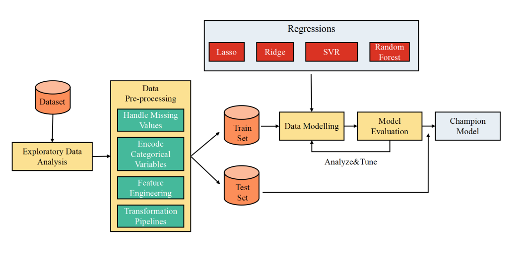
Figure 1: Modeling process diagram.

3. Experimental Process

3.1. Data Analysis and Visualization

3.1.1. Total Number of Samples and Features

This paper participated in the house price prediction competition on Kaggle [11] and obtained the competition dataset. According to the statistical results, the total number of samples in the training set is 2460, and each sample has a total of 81 features. Except for the “Id” feature and the label “SalePrice” of the training samples, each sample has 79 features.

3.1.2. Distribution of the SalePrice Label

First, the label of the training samples, which is the sale price of the houses, is extracted. From the basic statistics, it can be observed that the mean of the house sale prices is 180,921, with a minimum value of 34,900 and a maximum value of 755,000. To visually represent the distribution of house sale prices, a density plot of the sample house sale prices is shown in Figure 2.

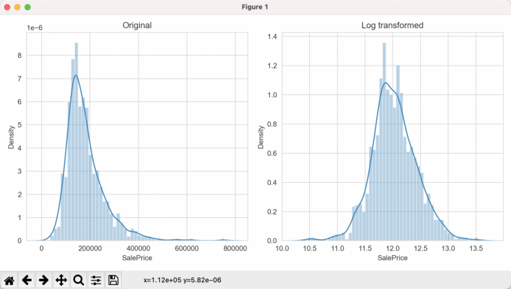
Figure 2: Density plot.

3.1.3. Distribution of SalePrice with YearBuilt

Among the numerous features, the year of construction (YearBuilt) is selected for analysis. Intuitively, it is generally believed that newer houses are more expensive than older houses. The visualization plot of the relationship between house sale prices and the year of construction is shown in Figure 3. From the plot, the general trend does support this intuition. However, since the feature “YearBuilt” has a wide range of values (from 1872 to 2010), directly using one-hot encoding would result in sparse features. Therefore, in the feature engineering phase, this feature will be digitally encoded.

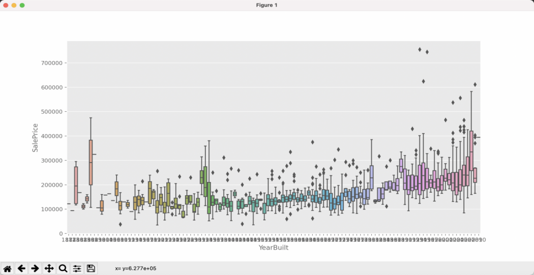
Figure 3: Distribution of SalePrice with YearBuilt.

3.1.4. Variation of SalePrice with GriLivArea

The living area of the house is also a crucial feature of the house. Intuitively, it is expected that the larger the living area, the higher the sale price. The variation of house sale prices with the living area (GriLivArea) is shown in Figure 4. From the figure, it can be observed that two points, located to the right of 4000 on the x-axis and below 200,000 on the y-axis, deviate from the common trend. Therefore, these samples with unconventional values will be removed from the training data.

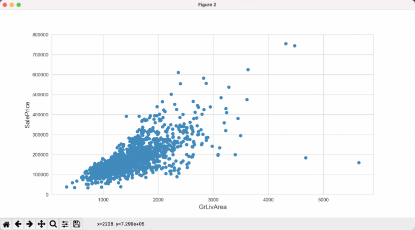
Figure 4: Variation of SalePrice with GriLivArea.

3.1.5. Variation of SalePrice with Other Important Features

In addition to the two fundamental features mentioned above, there are also many other important features. Although these important features are not analyzed one by one, their relationship with SalePrice is roughly understood to assist in subsequent feature engineering. The heatmap composed of the co-occurrence matrix. Additionally, to visually observe the relationship between SalePrice and these important features pairwise, a pairplot is plotted for the feature-label relationship. The selected important features for this visualization are OverallQual, GrLivArea, GarageCars, TotalBsmtSF, FullBath, and YearBuilt.

3.2. Data Cleaning

3.2.1. Missing Value Statistics for Features

The main task of data cleaning is to handle missing values. First, check the missing values for each feature.

3.2.2. Missing Value Imputation for Features

By carefully examining the content in the data description, it can be noticed that many missing values can be explained. For example, the first feature in the table, “PoolQC,” represents the quality of the pool. A missing value indicates that the house itself does not have a pool, so it can be filled with “None”. The provided Table 1 summarizes important information regarding various features in a dataset related to housing properties. The table outlines specific features that are to be filled with “None” if missing, indicating the absence of certain amenities like pools, miscellaneous features, alleys, fences, fireplaces, and specific garage or basement qualities and finishes. Additionally, features representing areas, such as “TotalBsmtSF” (total basement area) and others, will have their missing values filled with 0 if the corresponding property does not have a basement.

Table 1: Missing value imputation for features.

The feature “LotFrontage” has a significant relationship with “LotAreaCut” and “Neighborhood”. Here, the statistical data of “LotAreaCut” and “Neighborhood” are summarized. Therefore, the missing values in “LotFrontage” can be imputed using the median value based on the groups formed by these two features.

3.3. Feature Engineering

3.3.1. Ordinal Encoding for Categorical Variables

For ordinal encoding of categorical variables, the “get dummies” function in pandas can be used to convert them into numerical values. However, in this competition, simple one-hot encoding may not be enough. Therefore, the method used here is to group the features and calculate the average and median sale prices for each value of the feature. Then, the values are sorted and assigned based on these statistics. Taking the feature “MSSubClass” as an example, the data is grouped by this feature.

3.3.2. Feature Combination

Combining original features can often produce unexpected effects. However, since there are many original features in this dataset, it is not feasible to combine all of them. Therefore, Lasso is used for feature selection to choose some important features for combination. The importance of features is shown in Figure 5.

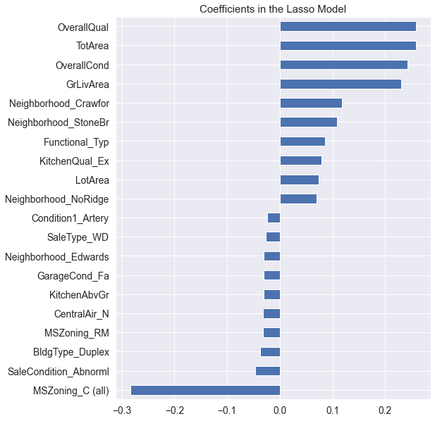
Figure 5: Feature importance ranking.

3.4. Modeling

3.4.1. Evaluation Metric

Before modeling, it is necessary to understand the evaluation metric for the problem. The evaluation metric for house price prediction is root mean squared error (RMSE), which is commonly used for regression problems. It is defined as follows:

RMSE = \( \sqrt[]{\frac{\sum _{i=1}^{N}{({y_{i}}-{\hat{y}_{i}})^{2}}}{N}} \)

When it comes to numerical prediction, the choice of models should not include classification models such as Support Vector Machines (SVM) or k-Nearest Neighbors (k-NN). Instead, algorithms like linear regression and random forest regression should be chosen for predicting house prices.

The modeling part involves building models based on the engineered features. In the case of regression problems, regression models are used. The following are the candidate models in this part: Lasso,Ridge,SVR,Random Forest.

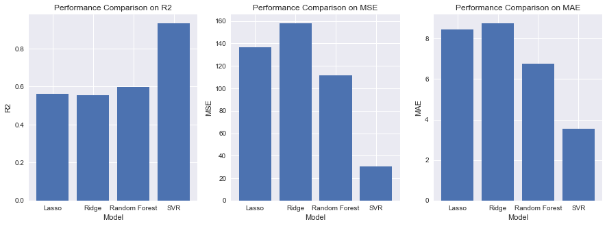
Figure 6: Result on validation set.

Next, this paper performed hyperparameter tuning for different models, using Lasso, Ridge, SVR, and Random Decision Trees as the base models.

Since the test results are only available on Kaggle and are automatically evaluated, the final RMSE experimental result submitted to the Kaggle leaderboard is 0.11981.

4. Conclusion

4.1. Results Analysis

During the experiment, missing values in the data were handled, and the experimental data was transformed to approximate a normal distribution to make the results more reasonable. In the process of trying out these functions separately, this paper did not use ensemble combinations but chose a single algorithm for regression prediction. This was mainly to understand the principles of each algorithm and to appreciate the impact of parameter settings on the results, rather than simply reducing loss and improving scores.

The final RMSE result was 0.11981, which is already very good considering only using machine learning. It is believed that most of the improvements should be attributed to data analysis and feature engineering, rather than the final model. After data cleaning and feature analysis in the preliminary stage, the results were excellent regardless of the chosen model. This indicates that the selected features have a strong correlation with the outcome, and the model has achieved the expected performance.

4.2. Improvement Expectations

(1) Model Stacking: Model stacking is a method for improving the performance of regression models. This technique combines the predictions of multiple models.

(2) Neural Networks: Neural networks can be considered as another method to enhance regression models. Neural networks have a powerful representation that captures complex relationships in the data.

4.3. Insights

(1) By analyzing the feature selection and attribute ranking, the main factors affecting the house price can be found. From the attribute ranking, it can be seen that people pay most attention to factors such as the quality of the house, the large area, and the good living environment when purchasing a house.

(2) The application of data analysis and machine learning methods can provide a scientific basis for house price prediction and reduce subjective judgment and randomness.

References

[1]. Jiang, J., & Liu, Y. (2016). A comparative study of machine learning methods for housing price prediction. Expert Systems with Applications, 60, 93-106.
[2]. Al-Mezel, S., Al-Dawood, M., & Al-Ajlan, S. (2012). Predicting House Prices Using Multiple Linear Regression Models. International Journal of Computer Science Issues (IJCSI), 9(2), 1-5.
[3]. Pramanik, S., Chow, U. N., Pram, B. K., & et al. (2010). A Comparative Study of Bagging, Boosting and C4.5: The Recent Improvements in Decision Tree Learning Algorithm. Asian Journal of Information Technology, 9(6), 300-306.
[4]. Tahir, Y., Tawab, T., Javed, S., & Naeem, M. (2018). House Price Prediction Using Machine Learning Techniques. International Journal of Computer Science and Network Security (IJCSNS), 18(1), 30-35.
[5]. Gu, X., & Li, C. (2012). House Price Prediction Research Based on Markov Chain. Consumer Economics, 2012(5), 4.
[6]. Hilber, C. A., & Vermeulen, W. (2016). The impact of supply constraints on house prices in England. The Economic Journal, 126(591), 358-405.
[7]. Gyourko, J., Mayer, C., & Sinai, T. (2013). Superstar cities. American Economic Journal: Economic Policy, 5(4), 167-199.
[8]. Dreger, C., & Kholodilin, K. A. (2013). An Early Warning System to Predict the House Price Bubbles. Social Science Electronic Publishing, 7(2013-8), 1-26. DOI:10.2139/ssrn.1898561.
[9]. Hayes, A. F. . (2013). Introduction to Mediation, Moderation, and Conditional Process Analysis: A Regression-Based Approach.
[10]. Breiman, L. I. , Friedman, J. H. , Olshen, R. A. , & Stone, C. J. . (2015). Classification and regression trees. Encyclopedia of Ecology, 57(3), 582-588.
[11]. Montoya, A., DataCanary, & et al. (2016). House Prices - Advanced Regression Techniques [Z]. Retrieved from https://kaggle.com/competitions/house-prices-advanced-regression-techniques.
Cite this article
Zong,Y. (2023). House Prices Prediction – Advanced Regression Techniques. Advances in Economics, Management and Political Sciences,50,181-189.
Data availability
The datasets used and/or analyzed during the current study will be available from the authors upon reasonable request.
Disclaimer/Publisher's Note
The statements, opinions and data contained in all publications are solely those of the individual author(s) and contributor(s) and not of EWA Publishing and/or the editor(s). EWA Publishing and/or the editor(s) disclaim responsibility for any injury to people or property resulting from any ideas, methods, instructions or products referred to in the content.
About volume
Volume title: Proceedings of the 2nd International Conference on Financial Technology and Business Analysis
© 2024 by the author(s). Licensee EWA Publishing, Oxford, UK. This article is an open access article distributed under the terms and
conditions of the Creative Commons Attribution (CC BY) license. Authors who
publish this series agree to the following terms:
1. Authors retain copyright and grant the series right of first publication with the work simultaneously licensed under a Creative Commons
Attribution License that allows others to share the work with an acknowledgment of the work's authorship and initial publication in this
series.
2. Authors are able to enter into separate, additional contractual arrangements for the non-exclusive distribution of the series's published
version of the work (e.g., post it to an institutional repository or publish it in a book), with an acknowledgment of its initial
publication in this series.
3. Authors are permitted and encouraged to post their work online (e.g., in institutional repositories or on their website) prior to and
during the submission process, as it can lead to productive exchanges, as well as earlier and greater citation of published work (See
Open access policy for details).