1. Introduction

Portfolio management is a very important topic of finance [1-3]. It can help investors choose better stock combinations to get more returns in the market [4-6]. This article is mainly about an investigation on finding the most efficient portfolio within 10 stocks. These 10 stocks are chosen from the S&P 500 and all of them are of great importance in their own industry. These 10 stocks are 3M, P&G, Disney, Activation Blizard, Lockheed Martin, J.P. Morgan, Nike, Tesla and Netflix. This investigation that aims to find such optimized portfolio from these 10 stocks could be a great application of portfolio management related knowledge.

In this article, data about these 10 stocks will be collected and processed. Then, the most efficient portfolio can be calculated using these data and Markowitz’s model. Excel solver would be used as a tool to testify the result.

2. Data Collection and Processing

This part will introduce how data for these stocks is collected and processed.

2.1. Target Stock Selection

For this project, I have selected 10 companies from different industries in the United States to find an optimal portfolio for these companies. All of these companies are members of the S&P 500 [7]. Here is a list of my choices of companies:

3M: 3M is known for its culture of innovation and investment in research and development. It made great efforts the invent innovative products; for example, adhesive tape, audio-visual equipment, and medical products. Thus, its stock is a good choice for research. Here is a stock price graph for 3M in the last 10 years.

Figure 1: 3M stock price graph.

Figure 1 shows that the increase generally increased from 2013 to 2018, and decreased from 2018 to 2020. Then, increased slightly in 2021 but started to decrease since then.

P&G: P&G is a manufacturer of daily products such as baby care, feminine care, cleaners, etc. It is one of the biggest enterprises in this area in the United States. Here is the stock price for P&G in the last 10 years.

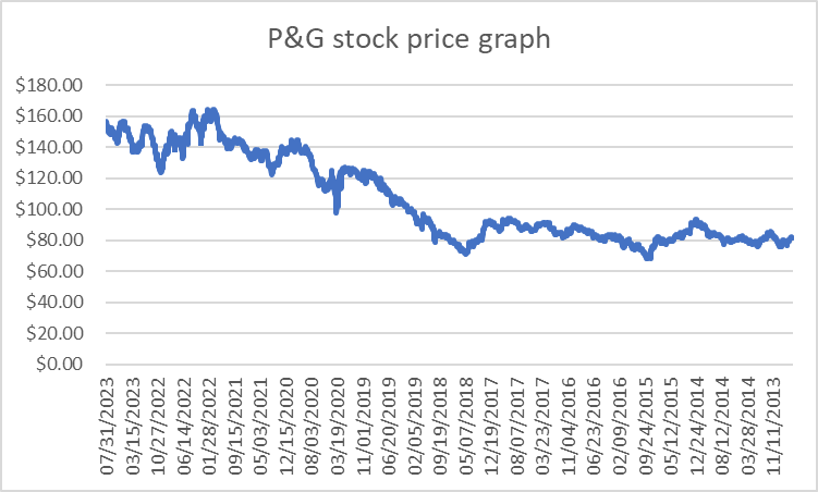
Figure 2: P&G stock price graph.

Figure 2 shows that the stock price of P&G generally increased within the last 10 years with some slight decrease from time to time

Disney: Disney is a corporation that covers areas like entertainment, theme parks, movies, etc. Its theme parks are all around the world which makes it the largest corporation in the entertainment industry. Here is the stock price for Disney in the last 10 years.

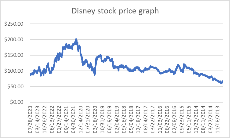
Figure 3: Disney stock price graph.

Disney’s stock price with stable from 2013 to 2019 while there was a sharp increase from 2020 to 2021 (Figure 3).

Activation Blizard: Activation Blizard is one of the most successful interactive entertainment and gaming corporations in the world. Here is the stock price for Blizard in the last 10 years (Figure 4).

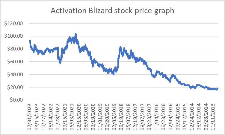
Figure 4: Activation Blizard stock price graph.

Activation Blizard’s stock price increased slightly from 2013 to 2018 while it fell dramatically in 2018 and recovered in 2020.

Lockheed Martin: Lockheed Martin is a global-leading security and aerospace. It mainly covers 4 areas: Aeronautics, Missiles and fire control, rotary and mission systems, and space. Here is the stock price for Lockheed Martin in the last 10 years.

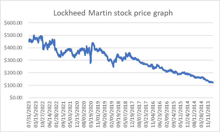
Figure 5: Lockheed Martin stock price graph.

Lockheed Martin’s stock price increased gently but also consistently in the last ten years with some fluctuation from 2018 to 2020 (Figure 5).

American Electric Power: American Electric Power offers gas and electricity for families all over the United States. It produces power using coal, lignite, natural gas, etc. Here is the stock price for American electric power in the last 10 years (Figure 6).

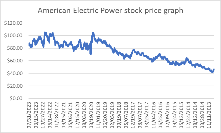
Figure 6: American electric power stock price graph.

American Electric Power’s stock price increased from 2013 to 2019 but fell sharply in 2019 and fluctuated around $90 since then.

J.P. Morgan: J.P. Morgan is a financial holding company that offers consumer and commercial banking, investment banking, financial transaction processing, and asset management solutions through its subsidiaries. Here is the stock price for J.P. Morgan in the last 10 years (Figure 7).

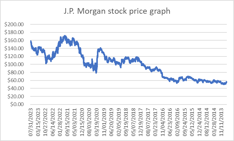
Figure 7: J.P Morgan stock price graph.

J.P Morgan’s stock price trend was similar to previous stocks, increased from 2013 to 2019, and fell in 2019 while recovering in the following years.

Nike: Nike is a multinational corporation that manufactures and sells footwear, apparel, equipment, accessories, and services. Here is the stock price for Nike in the last 10 years (Figure 8).

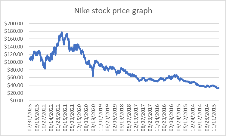
Figure 8: Nike stock price graph.

Nike’s stock increased slightly from 2013 to 2019, to around $100. Then, it sharply increased from 2019 to 2022 with the highest price of around $180 but decreased to $100 from 2022 to 2023.

Tesla: Tesla engages in the design, development, manufacture, and sale of fully electric vehicles, energy generation and storage systems. It also offers a supercharger station and self-driving capability. Here is the stock price for Nike in the last 10 years (Figure 9).

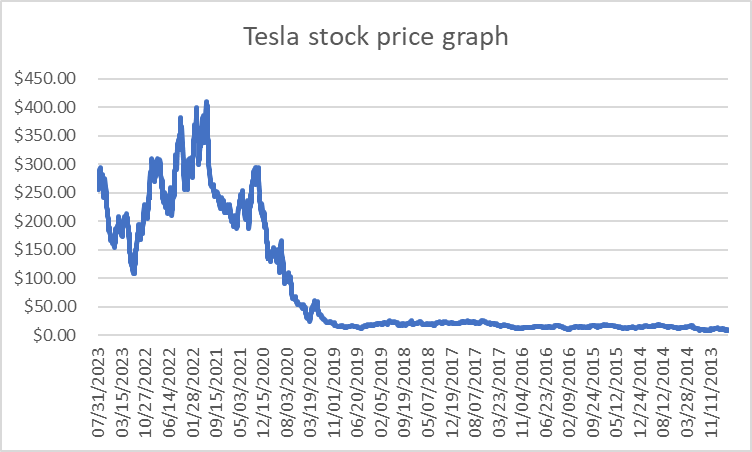
Figure 9: Tesla stock price graph.

Tesla’s stock price was very low from 2013 to 2020 and dramatically increased to $400 in 2021 but decreased the next year.

Netflix: Netflix is a streaming entertainment service company, which offers subscription service for streaming movies and TV shows. Here is the stock price for Netflix in the last 10 years (Figure 10).

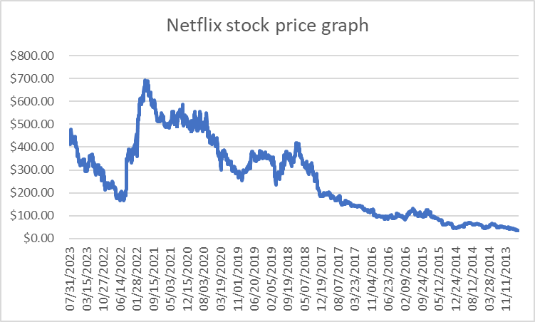
Figure 10: Netflix stock price graph.

Netflix’s stock price increased from $70 to $700 from 2013 to 2021 while decreasing back to $200 in 2022. It recovered to $460 this year.

2.2. Model Introduction

With these choices of companies and stock prices collected as shown in the graph, we can use the Markowitz model to optimize our portfolio. Using this model, it is possible to find optimal weightings for each stock.

Markowitz model, which is also known as mean-variance model, is a portfolio optimization model [7-9]. Using this model, we analyze various conditions for various expected returns (mean) and variances for different portfolios to maximize our “return-to-risk” ratio, which in other words, the Sharpe ratio.

Applying our data of stock price into this model to optimize our portfolio:

Firstly, from the data of stock price for each month, we can calculate a monthly expected return for 10 companies. The equation is shown below

\( \frac{{P_{a}}-{P_{a-1}}}{{P_{a-1}}} \) (1)

where \( {P_{a}} \) is the stock price for this month and \( {P_{a-1}} \) is the stock price for last month. Thus, the rate of return for every week is calculated. Then, the average rate of return can be calculated using Excel:

Table 1: Average return and standard deviation.

These are important data to calculate the covariance matrix for the rate of returns.

To calculate the covariance matrix [10], we first use Excel to come up with a matrix D, where all elements in this matrix are calculated in the following formula:

\( \frac{{R_{n}}-E(R)}{\sqrt[]{N}} \) (2)

where \( {R_{n}} \) is the corresponding rate of return for a certain month and \( E(R) \) the average rate of return for this stock. \( N \) is the number of data, which in this case is the number of months in 10 10-year period.

After calculating the matrix D, based on the definition of covariance and the previous formula, we multiply the transpose of it by itself to get the covariance matrix.

\( Cov(x,y)=\frac{\sum (X-E(X))(Y-E(Y))}{N} \) (3)

\( C={D^{T}}D \) (4)

The covariance matrix of the rate of return is shown below:

Table 2: Covariance matrix.

After this, the expected return should be collected. Although the average rate of return seems a good source for the expected return, it is not a reliable estimation for the expected return in the future, which is very important in further calculations. Thus, data that is predicted by experts from TIPRANKS are used in this calculation.

Then, all these data can be used to calculate the most efficient portfolio.

Using indexes about efficient frontier for a given R, where

\( A={1^{ \prime }}{Σ^{-1}}1 \) (5) \( B={1^{ \prime }}{Σ^{-1}}r \) (6) \( C={r^{ \prime }}{Σ^{-1}}r \) (7) \( D=AC-{B^{2}} \) (8)

All of these values, A, B, C, and D are used to minimize the risk, in this case, the variance for our data. This variance should be on our efficient portfolio frontier. The processed variance can be calculated with the following formula:

\( {σ^{2}}=\frac{A{R^{2}}-2BR+C}{D} \) (9)

In these formulas, \( Σ \) stands for the covariance matrix while r is the future expected return. Based on this variance, the following formula can be used to calculate the weighting of the most efficient portfolio.

3. Result

Here is the most efficient portfolio weighting and its corresponding risk (Table 3).

Table 3: Result and risk.

To test the accuracy of this result, an alternative method is used to calculate this weighting. Solver in Excel can be used to calculate this weighting.

The weighting calculated using the solver is:

Table 4: Solver calculated weight.

This is the weighting calculated from the Excel solver (Table 4), which is the same as our previous result. This proves that this weighting is accurate. Also, using this solver, we can set some constraints to the weighting, such as all of the weightings should be greater or equal to zero (Table 5). (As shown below)

Table 5: Weighting with constraints.

4. Conclusion and Reflection

4.1. Background and Methodology

The idea of this portfolio management comes from a project together with my classmates. We had just learned about portfolio management and decided to use the Markowitz model to calculate the most efficient portfolio for some companies that we are interested in. All of the companies chosen are in the S&P 500, which is an essential index. When choosing these target stocks, we a wide range of companies and eliminated most of them with only 10 representative companies left for investigation.

4.2. Results Analysis

For the result calculated, we can make some conclusions about the weightings calculated. Disney, American Electric Power, and Nike are positive in weighting in our most efficient portfolio. This result is reasonable since these three have higher future expected returns, which reflect its higher possible return in this case. Also, after setting the constraints to the Excel solver which lets all of the weighting be greater or equal to zero, only these three stocks have positive weighting which is consistent with the previous result. For this portfolio, we have a Sharpe ratio of 42.5% and 31.1% with constraint, which is a very high Sharpe ratio for a portfolio, this number reflects that this portfolio is successful. For the expected return, the former portfolio gives a 16.2% expected return while constrained weighting only gives a 2.3% future expected return. Optimization gives a very impressive expected return for the weighting, however, the real situation would be far more complex and a 16% monthly expected return is impossible.

4.3. Errors and Further Development

When collecting data for the future expected return, many more choices can be used. For example, CAPM is a very feasible way to calculate future expected returns for those stocks.

\( r={r_{f}}+β({r_{m}}-{r_{f}}) \) (10)

This is a formula for CAPM calculation. However, the choice of market return will still be a problem and might cause biased calculations. On the other hand, the calculation of beta values based on all given data was difficult. This is the reason that an expert’s prediction is used to future expected returns.

For the result calculated from optimization, the expected return was way higher than expected. This should be because we used an expert’s prediction on future expected returns. The real expected return should be more complex. On the other hand, expected returns calculated for constrained weighting were more reasonable. This might imply that not all portfolio weightings are possible in real life. Instead, adding some constraints would help the calculation closer to reality.

References

[1]. Wang Lei, Bao Xinzhong. Research on patent portfolio value assessment based on fuzzy hierarchical analysis and real option method[J]. China Invention and Patent, 2022, 19(8):10.
[2]. Yuenan Wang, Amalia Di Iorio, The cross section of expected stock returns in the Chinese A-share market, Global Finance Journal, Volume 17, Issue 3, 2007, Pages 335-349, ISSN 1044-0283.
[3]. Hua, R., & Chen, B. International linkages of the Chinese futures markets[J]. Applied Financial Economics, 2007, 17(16), 1275-1287.
[4]. Cassimon D , Engelen P J , Thomassen L ,et al. The valuation of a NDA using a 6-fold compound option[J].Research Policy, 2004, 33(1):41-51.DOI:10.1016 /s0048-7333(03)00089-1.
[5]. Zhu B. A comparative study of gains and losses of European-style portfolio options[J]. Enterprise Economics, 2006(7):3. DOI:10.3969/j.issn.1006-5024.2006.07.031.
[6]. Y. Xu. Portfolio option pricing with information influence based on fractional Brownian motion[J]. Practice and Understanding of Mathematics, 2014(19):6. DOI:CNKI:SUN:SSJS.0.2014-19-021.
[7]. TANG Mingkun, FENG Zhenhua, ZHAO Zhenyu. Research on option portfolio arbitrage under Bayesian game framework; Theoretical model and market data validation[J]. Southern Economy, 2023(4):79-97.
[8]. Whaley, R. E. Valuation of American futures options: Theory and empirical tests[J]. The Journal of Finance, 1986, 41(1), 127-150.
[9]. Thomassen L , Van W M .The n-fold compound option[J]. martine van wouwe, 2001.DOI:http://dx.doi.org/.
[10]. Zhao P , Wang T , Xiang K ,et al. N-Fold Compound Option Fuzzy Pricing Based on the Fractional Brownian Motion[J]. Systems, 2022.DOI:10.1007/s40815-022-01283-2.
Cite this article
Wu,C. (2023). Investigation of Optimizing Portfolio for Ten Chosen Stocks. Advances in Economics, Management and Political Sciences,53,99-109.
Data availability
The datasets used and/or analyzed during the current study will be available from the authors upon reasonable request.
Disclaimer/Publisher's Note
The statements, opinions and data contained in all publications are solely those of the individual author(s) and contributor(s) and not of EWA Publishing and/or the editor(s). EWA Publishing and/or the editor(s) disclaim responsibility for any injury to people or property resulting from any ideas, methods, instructions or products referred to in the content.
About volume
Volume title: Proceedings of the 2nd International Conference on Financial Technology and Business Analysis
© 2024 by the author(s). Licensee EWA Publishing, Oxford, UK. This article is an open access article distributed under the terms and
conditions of the Creative Commons Attribution (CC BY) license. Authors who
publish this series agree to the following terms:
1. Authors retain copyright and grant the series right of first publication with the work simultaneously licensed under a Creative Commons
Attribution License that allows others to share the work with an acknowledgment of the work's authorship and initial publication in this
series.
2. Authors are able to enter into separate, additional contractual arrangements for the non-exclusive distribution of the series's published
version of the work (e.g., post it to an institutional repository or publish it in a book), with an acknowledgment of its initial
publication in this series.
3. Authors are permitted and encouraged to post their work online (e.g., in institutional repositories or on their website) prior to and
during the submission process, as it can lead to productive exchanges, as well as earlier and greater citation of published work (See
Open access policy for details).