


1. Introduction
The electric vehicle (EV) industry, once a niche market, has rapidly evolved into a major player in the global automotive sector. As environmental concerns intensify and nations grapple with the challenges of climate change, the push for sustainable and eco-friendly transportation solutions has gained unprecedented momentum. Traditional gasoline-powered vehicles, with their significant carbon footprints, are gradually giving way to their electric counterparts. Leading this charge are companies like Tesla and NIO, which have not only redefined automotive engineering but have also reshaped the financial landscape with their impressive market valuations.
The rise of the EV market is not solely an outcome of environmental imperatives [1]. This case is also an interesting illustration of the ways in which the reduction of life-cycle carbon emissions attributable to the use phase (currently circa 85 % for a standard car) throws increased attention on the carbon cost of manufacturing, and hence the need to mitigate emissions in this area. Technological advancements, particularly in battery storage and charging infrastructure, have played a pivotal role in making EVs more accessible and appealing to the average consumer. Furthermore, changing consumer preferences, driven by a heightened awareness of environmental issues and the allure of innovative tech integrations, have further bolstered the EV market's growth.
However, with growth comes volatility, especially in the financial markets. The stock prices of major EV manufacturers, such as Tesla and NIO, have been the subject of much speculation and analysis. Their performance in the stock market offers insights not just into the companies' health but also into broader market perceptions and future industry trends. This essay delves deep into a sensitivity analysis of these two giants in the EV industry, aiming to shed light on the dynamics of their stock prices and the implications these have for potential investors. Through a meticulous examination of stock and option prices, this study seeks to provide a comprehensive understanding of the investment landscape in the burgeoning world of electric vehicles.
2. Data Preparation
2.1. Data Collection
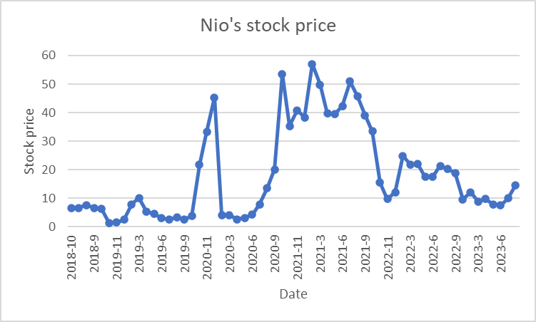
Figure 1: Nio’s stock price.
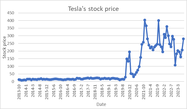
Figure 2: Tesla’s stock price.
One of the pivotal aspects of this analysis was the collection of daily stock prices for both Tesla and NIO. We tried to find some ways, to ensure that the data was both accurate and comprehensive. By leveraging various financial databases and platforms, we were able to compile a dataset that spanned a significant timeframe, providing a holistic view of the stock price movements. The stock price may be independent so we only apply it to the Sensitivity analysis [2]. The weak form hypothesis in the market implies that successive stock price changes are independent and identically distributed, so the past movements or trends of a stock price or market cannot be used to predict its future movements (Figures 1 and 2).
2.2. Monthly Return Calculation
After obtaining the daily stock prices, the next step was to compute the monthly returns. This is crucial as monthly returns provide a more aggregated view of stock performance, smoothing out daily volatilities and offering a clearer picture of longer-term trends. Using Microsoft Excel, I employed the formula:
Monthly Return= [(Start of Month Price-End of Month Price)/Start of Month Price] ×100(1)
The stock return is defined as the logarithm of monthly price difference [3].
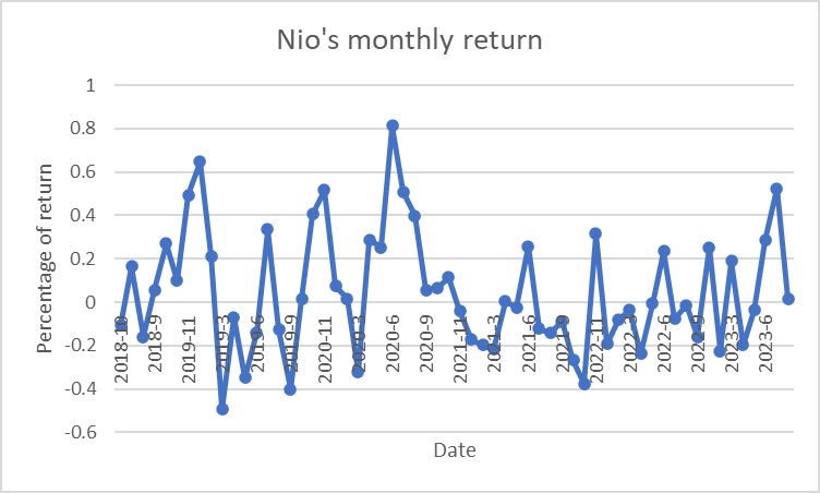
Figure 3: Nio’s monthly return.
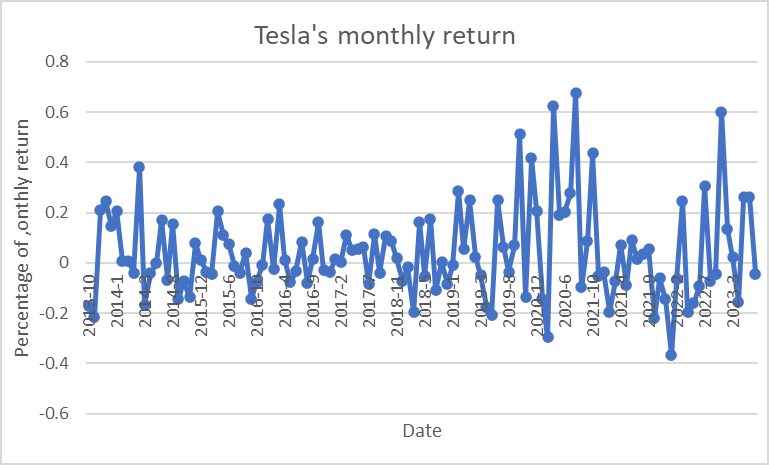
Figure 4: Tesla’s monthly return.
This formula helped in determining the percentage change in stock price over each month, which was then used for further analysis and the dividend payment should be accounted for (Figures 3 and 4).
2.3. Option Analysis
In addition to stock prices, we delved into the world of options, specifically focusing on Tesla and NIO. Options, being derivative instruments, derive their value from the underlying asset, in this case, the stocks of Tesla and NIO. We collected data on the strike prices of these options, which is the predetermined price at which the holder can buy or sell the underlying stock. [4]Option chain analysis involves studying the available options contracts for an underlying asset, such as a stock, commodity, or index. An option chain provides a detailed list of all the calls and put options available for a given security.
Furthermore, we gathered information on the volatility of these options. Volatility, in the context of options, refers to the degree of variation of the option's price over time and is a crucial determinant of the option's value.
Lastly, we recorded the stock prices of Tesla and NIO at specific timestamps. This data, combined with the strike price and volatility, provides a comprehensive view of the option's intrinsic and time value, aiding in the overall sensitivity analysis.
3. Introduction to the Model
3.1. Combination Option Models
\( {S_{t}}={S_{0}}*{e^{(r-q-0.5*{σ^{2}})*t+{Z_{1}}*σ*\sqrt[]{t}}} \) (2)
Individual variables and meanings:
\( {S_{t}} \) : This is the price of the underlying asset at the time the option expires. At the expiration of the option, if the price of the underlying asset is higher than the strike price, the investor holding the option can exercise the option to gain a profit.
\( {S_{0}} \) : This is the initial underlying asset price of the option, i.e. the price of the underlying asset at the time of the option purchase.
\( e \) : This is the base of the natural logarithm, i.e., it is approximately equal to 2.71828.
\( r \) : This is the risk-free rate, which represents the rate of return that would be earned on the funds in the absence of risk. The risk-free rate is often used as an important variable in option pricing models.
\( q \) : This is the dividend yield of the underlying asset and represents the dividends paid on the underlying asset during the option holding period.
\( 0.5*{σ^{2}} \) : This component represents half of the square of the volatility of the underlying asset price. Half the square of volatility is often used to measure the volatility of an option price.
\( t \) : This is the holding time of the option and indicates the length of time from the time the option was purchased to expiration.
\( {Z_{1}} \) : This is a random variable that follows a standard normal distribution and is used to represent the uncertainty of option price fluctuations.
\( σ \) : This is the volatility of the price of the underlying asset, which, as mentioned earlier, measures the degree of volatility of the price of the underlying asset.
\( \sqrt[]{t} \) : This is the square root of \( t \) the square root of the square root of the square root of the square root of the square root of the option holding time.
Equation (2) above describes the change in the price or value of a portfolio option, which includes the effects of changes in the price of the underlying asset, the risk-free rate, the dividend yield, the volatility of the underlying asset, and time. Such a model can be used for option pricing and risk management [5].
3.2. Truncated Course
\( {K^{*}}=K*{e^{-r*(T-t)}} \) (3)
Equations (3) above describe a truncated (truncated) towards (forward) calculation that involves the following variables:
\( {K^{*}} \) : This is the value calculated by truncating the direction of travel.
\( K \) : This is the initial value.
\( e \) : This is the base of the natural logarithm, i.e., it is approximately equal to 2.71828.
\( r \) : This is the risk-free rate, which represents the rate of return that could have been earned on the funds in the absence of risk. \( r \) The difference multiplied by time ( \( T-t \) ) indicates the interest accrued during this period.
\( T \) : This is the end time of the truncation.
\( t \) : This is the start time of the truncation.
The purpose of Equation (3) is to calculate the risk-free rate at the cut-off time \( T \) after which the specified risk-free rate \( r \) The initial value when discounting is carried out \( K \) of the case. In other words, it takes the initial value \( K \) based on the risk-free rate \( r \) Discounting is performed to extend the time from \( t \) extending the time from \( T \) , obtaining a truncated value of \( {K^{*}} \) .
In finance, this truncated heading calculation is commonly used to calculate the present value of financial instruments, especially for discounting future cash flows [6]. This is used in areas such as option pricing, bond valuation, and financial derivatives. The truncated path calculation is able to take into account the effect of the risk-free rate on the time value of money, thus obtaining the present value at a future point in time. \( T \) present value at a future point in time. This is important for risk management, investment decisions and asset pricing (Figure 5).
 Figure 5: Schematic diagram of cut-off time.
3.3. Option Execution Judgement
\( St \gt {K^{*}} \) : Choice to exercise options(4)
\( St \lt {K^{*}} \) : Choice not to exercise option(5)
Equations (4) and (5) describe an option's exercise rule, based on a comparison of the price of the underlying asset and the truncated move to decide whether to exercise the option. Let us explain each of these components in turn:
\( St \) :This is the price of the underlying asset at the time the option expires. At option expiration, we observe the actual price of the underlying asset.
\( {K^{*}} \) : This is the value of the truncation towards the calculation obtained from the previous calculation. In the previous formula, we calculated the truncation time at the truncation time \( T \) After that, based on the risk-free rate \( r \) Discounting the initial value \( K \) The truncated value obtained by discounting it.
Based on the comparison of the above two values, two cases are included in Eq:
If the price of the underlying asset \( St \) is greater than the cut-off value \( {K^{*}} \) , then the execution rule for the option is: exercise the option (i.e., choose to execute the option). This means that the investor holding the option can, at the strike price \( K \) purchase the underlying asset and can then sell it immediately for a profit because the market price is higher than the strike price.
If the price of the underlying asset \( St \) is less than the cut-off value \( {K^{*}} \) , then the execution rule of the option is: do not exercise the option (i.e., choose not to execute the option). This means that the investor holding the option will not purchase the underlying asset through the option because the market price is lower than the strike price.
The purpose of this rule is to help investors make decisions about whether to exercise an option. By comparing the price of the underlying asset to a truncated value obtained by discounting the risk-free rate, investors can decide whether or not to exercise the option to maximise their benefits based on market realities [7]. This type of decision making is very common in options trading as it relates to whether or not an investor should use an option to make a potential profit.
4. Analysis Using Tesla and Azera as Examples
4.1. Correlation Coefficient
Tesla option stock price parameters: s0 = 267.43; k = 270; r = 4.01%; q = 0; volatility σ = 36.73%; t is assumed to be 0.5 years; t is assumed to be 1 year.
Parameters of Azure option stock price:, S0 = 14.82; K = 15; r = 4.01%; q = 0; volatility σ = 41.21%; t is assumed to be 0.5 years; T is assumed to be 1 year.
The results of the calculations are shown in Table 1.
Table 1: Tesla Options Stock Price Analysis.
Stock Name | Call Option Price | Put Option Price | Chooser Price | Straddle Price |
Nikola Tesla (1856-1943), Serbian inventor and engineer | 18.75 | 11.75 | 15.25 | 30.5 |
Ulai Motors (car manufacturer) | 1.37 | 1.18 | 1.275 | 2.55 |
4.2. Sensitivity Analysis
It is assumed that the share prices of both Tesla and Azera gradually increase from a low level, so as to observe the change of Chooser's price. The specific calculation results are shown in Figure 6 and Figure 7.
Figure 6: Changes in Tesla Chooser Prices.
We can observe the sensitivity of the Chooser option price to changes in the share price. Sensitivity analyses are conducted by selecting a few stock price data points in order to explore how the Chooser price responds to changes in the stock price. The specific data point changes are shown in Table2 below:
Determine the baseline data point in order to begin the sensitivity analysis. Among the above data, the data point with a stock price of 20.99 can be selected as the benchmark data point.
Table 2: Sensitivity analysis of Chooser's option price to changes in Tesla's share price.
equity price | Chooser Price | Percentage change |
20.99 | 0.03 | N/A |
95.38 | 3.85 | 11766.67 per cent |
164.31 | 16.45 | 327.27 per cent |
265.25 | 23.82 | 44.89 per cent |
371.33 | 35.67 | 49.78 per cent |
In this sensitivity analysis, we can see that as the share price increases, the Chooser price shows a significant increase. This suggests that the stock price has a strong positive sensitivity to the Chooser price, i.e., when the stock price increases, the Chooser price also increases[8]. This is intuitive because when the stock price is closer to the option strike price (K=270), the Chooser option is more valuable and investors are more willing to pay a higher price to get this option.
The changes in the Chooser price were observed at different volatility levels. Below are the results of selecting some volatility levels and calculating the corresponding Chooser prices. The volatility takes values ranging from 10 per cent to 50 per cent:
Table 3: Analysis of changes in Tesla's volatility.
Volatility (%) | Chooser price for shares (20.99) | Chooser price of the stock (371.33) |
10 | 0.00 | 1.07 |
20 | 0.02 | 10.24 |
30 | 0.05 | 25.50 |
40 | 0.08 | 44.46 |
50 | 0.11 | 68.73 |
From this analysis, it can be seen that as volatility increases, Chooser option prices increase overall. This is consistent with the volatility sensitivity in option pricing theory. When volatility increases, the uncertainty of the option increases and therefore investors place a higher value on the Chooser option. This trend holds for both the benchmark stock price (20.99) and the higher stock price (371.33) data points.
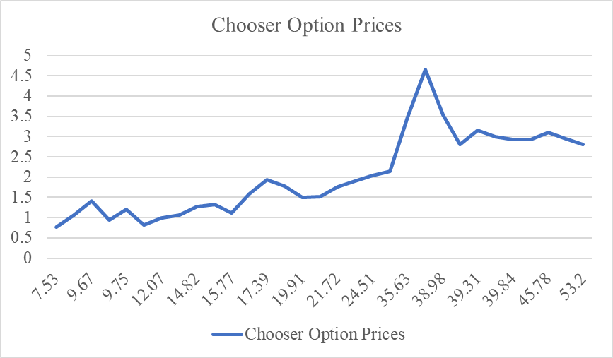
Figure 7: Changes in Azera's Chooser Price.
Choosing the stock price data point 7.53 as the baseline data point, we can calculate the percentage change in the Chooser price for each data point relative to the previous data point.
Table 4: Sensitivity analysis of Chooser's option price to changes in Azera's share price.
equity price | Chooser Option Prices | Percentage change |
7.53 | 0.77 | N/A |
9.39 | 1.065 | 38.05 per cent |
9.67 | 1.41 | 32.90 per cent |
9.69 | 0.945 | -32.62 per cent |
9.75 | 1.2 | 26.46% |
10.51 | 0.815 | -32.08 per cent |
12.07 | 0.985 | 21.00 per cent |
12.78 | 1.07 | 8.63 per cent |
14.82 | 1.275 | 19.16 per cent |
15.3 | 1.33 | 4.31 per cent |
15.77 | 1.11 | -16.54 per cent |
16.7 | 1.59 | 43.24 per cent |
17.39 | 1.93 | 21.38 per cent |
19.73 | 1.78 | -7.77 per cent |
19.91 | 1.49 | -16.85 per cent |
21.05 | 1.51 | 1.34 per cent |
21.72 | 1.76 | 16.56 per cent |
22.84 | 1.9 | 7.95 per cent |
24.51 | 2.03 | 6.84 per cent |
31.68 | 2.14 | 5.42 per cent |
35.63 | 3.49 | 63.55 per cent |
38.62 | 4.65 | 33.53 per cent |
38.98 | 3.53 | -24.00 per cent |
39.13 | 2.8 | -20.66 per cent |
39.31 | 3.16 | 12.86 per cent |
39.41 | 3 | -5.03 per cent |
39.84 | 2.93 | -2.33 per cent |
44.68 | 2.92 | -0.34 per cent |
45.78 | 3.1 | 6.16 per cent |
48.74 | 2.94 | -5.16 per cent |
53.2 | 2.8 | -4.76 per cent |
From the sensitivity analysis results, it can be observed that in some cases, the Chooser price shows positive sensitivity to share price changes, i.e., when the share price increases, the Chooser price increases as well, e.g., the share price is 9.39, 9.67, 9.75, and 12.07. However, there are also cases where the Chooser price shows negative sensitivity to share price changes, i.e., when the share price increases, the Chooser price decreases, e.g., share prices of 9.69, 15.77, 19.91, etc.
The results of this sensitivity analysis show that the response of Chooser's option prices to changes in share prices is not always consistent at different share price levels and may be affected by other factors. This further emphasizes the importance of integrating multiple factors in investment decisions.
There seems to be some correlation between stock prices and Chooser option prices, but it is not a perfectly positive relationship. As the stock price rises, the change in the Chooser option price is not linear [9].
When Azera's share price did not exceed $38, Chooser option prices trended upward as Azera's share price increased, but when Azera's share price exceeded $38, Chooser option prices declined relatively as Azera's share price increased, reflecting the market's expectation of the stock's future volatility.
Table 5: Volatility changes.
Volatility (%) | 7.53 | 12.07 | 19.73 | 31.68 | 53.2 |
10% | 0.81 | 1 | 1.72 | 2.23 | 3.01 |
20 per cent | 1.02 | 1.29 | 2.21 | 2.97 | 4.19 |
30 per cent | 1.31 | 1.64 | 2.83 | 3.76 | 5.31 |
40 per cent | 1.63 | 2.05 | 3.53 | 4.68 | 6.59 |
50% | 1.94 | 2.45 | 4.24 | 5.6 | 7.87 |
The results of the sensitivity analyses show that stock prices have different effects on Chooser option prices. In some cases, an increase in the share price leads to an increase in the Chooser price, while in other cases, an increase in the share price leads to a decrease in the Chooser price. This is due to changes in market conditions as well as other unconsidered factors.
Specific point of attention:
In the higher range of stock prices, such as over $35, Chooser option prices have greater volatility, which may be due to the increased volatility of the stock at this time and also reflects investor uncertainty about the market's direction.
The results of the sensitivity analyses for Tesla and Azera show the trend of Chooser option prices as a function of share price and volatility.
Tesla sensitivity analysis results:
Chooser option prices have a tendency to increase as the stock price rises. This indicates that the market is more consistent in its expectation of an increase in Tesla's stock price, and investors are more willing to buy Chooser options in this case.
Increased volatility can lead to higher Chooser option prices. This suggests that the market expects increased volatility in Tesla's stock price and that investors may be interested in options in a high-volatility environment.
Results of the sensitivity analysis for Azure:
For Azure, the overall trend shows that Chooser option prices increase with share price and volatility over a range, which is in line with the expectations of the option pricing model.
Status quo and decision-making factors facing investors:
Investors should keep an eye on changes in stock price and volatility. Buying Chooser options may be an effective strategy when investors anticipate an increase in Tesla or Azera's stock price, as an increase in the option price can provide greater potential returns.
Investors also need to keep an eye on market sentiment and news, as major events may affect stock prices and volatility. If a major announcement or event is anticipated that could cause dramatic stock price movements, investors may look to options for hedging or profit opportunities[10].
It is important to note that investing in options carries risks as options may lose their full value at expiry. Therefore, investors need to give due consideration to their risk tolerance, investment objectives, and time when making decisions. It is advisable to work out an investment plan with a professional financial advisor and use options as part of your investment strategy where appropriate.
5. Conclusion
Sensitivity analysis is an important tool in finance that helps investors understand the relationship between stock or option prices and key variables to make more informed investment decisions. This sensitivity analysis focuses on the response of Tesla and Azera's Chooser option prices to changes in stock price and volatility.
For Tesla, we have observed a trend of Chooser option prices rising with the stock price. There seems to be a general market expectation that Tesla's share price may rise, and investors may be inclined to purchase Chooser options to take advantage of the potential increase. At the same time, increased volatility has increased Chooser option prices, which may reflect the market's expectation of widening volatility in Tesla's stock price.
The general trend of the results of the sensitivity analysis for Azure shows that within a certain range, Chooser option prices increase with stock price and volatility. Despite the limited data, this is consistent with the general pattern of option pricing models that option prices are likely to increase in an environment of high share price and volatility.
For investors, the following points are worth noting and summarising:
Stock Price Trend: Observe the long-term trend of the stock price and determine the market's expectation of the company's future movements. Based on the trend, consider whether to purchase options.
Volatility: Watch for changes in stock price volatility. A high-volatility environment may increase the value of an option, but it also comes with higher risk.
Market Events: Dramatic changes in stock prices and Chooser option prices over a given time period may be related to market events. Watch for major announcements, earnings releases, and other information.
Risk Management: Sensitivity analyses provide additional information for investment decisions, but risk management is critical. The help of a professional financial advisor may be required to develop a wise investment plan based on your risk tolerance and investment objectives.
In conclusion, sensitivity analyses provide investors with more comprehensive market information, but investment decisions need to take into account a variety of factors and be cautious of risk in order to achieve long-term sound investment objectives.
Authors Contribution
All the authors contributed equally and their names were listed in alphabetical order.
References
[1]. Beeton, D. and Meyer, G. eds. (2015). Electric vehicle business models: global perspectives. Page 11.
[2]. Dritsaki , C. (2015). Box–Jenkins modeling of greek stock prices data. International journal of economics and financial issues, 5(3), pp.740–747.
[3]. Yuenan Wang, Amalia Di Iorio, The cross section of expected stock returns in the Chinese A-share market, Global Finance Journal, Volume 17, Issue 3, 2007, Pages 335-349, ISSN 1044-0283.
[4]. Published On March 8, 2021 and Last Modified On May 23rd, 2023 https://www.analyticsvidhya.com/blog/2021/03/stock-options-chain-analysis-using-excel/.
[5]. Zhu B. A comparative study of gains and losses of European-style portfolio options[J]. Enterprise Economics, 2006(7):3. DOI:10.3969/j.issn.1006-5024.2006.07.031.
[6]. Y. Xu. Portfolio option pricing with information influence based on fractional Brownian motion[J]. Practice and Understanding of Mathematics, 2014(19):6. DOI:CNKI:SUN:SSJS.0.2014-19-021.
[7]. TANG Mingkun, FENG Zhenhua, ZHAO Zhenyu. Research on option portfolio arbitrage under Bayesian game framework; Theoretical model and market data validation[J]. Southern Economy, 2023(4):79-97.
[8]. Wang Lei, Bao Xinzhong. Research on patent portfolio value assessment based on fuzzy hierarchical analysis and real option method[J]. China Invention and Patent, 2022, 19(8):10.
[9]. Thomassen L , Van W M .The n-fold compound option[J]. martine van wouwe, 2001.DOI:http://dx.doi.org/.
[10]. Zhao P , Wang T , Xiang K ,et al. N-Fold Compound Option Fuzzy Pricing Based on the Fractional Brownian Motion[J]. Systems, 2022.DOI:10.1007/s40815-022-01283-2.
Cite this article
Huo,W.;Wu,H. (2023). Sensitivity Analysis Based on Portfolio Option Models Using Tesla and Nio as Examples. Advances in Economics, Management and Political Sciences,53,110-120.
Data availability
The datasets used and/or analyzed during the current study will be available from the authors upon reasonable request.
Disclaimer/Publisher's Note
The statements, opinions and data contained in all publications are solely those of the individual author(s) and contributor(s) and not of EWA Publishing and/or the editor(s). EWA Publishing and/or the editor(s) disclaim responsibility for any injury to people or property resulting from any ideas, methods, instructions or products referred to in the content.
About volume
Volume title: Proceedings of the 2nd International Conference on Financial Technology and Business Analysis
© 2024 by the author(s). Licensee EWA Publishing, Oxford, UK. This article is an open access article distributed under the terms and
conditions of the Creative Commons Attribution (CC BY) license. Authors who
publish this series agree to the following terms:
1. Authors retain copyright and grant the series right of first publication with the work simultaneously licensed under a Creative Commons
Attribution License that allows others to share the work with an acknowledgment of the work's authorship and initial publication in this
series.
2. Authors are able to enter into separate, additional contractual arrangements for the non-exclusive distribution of the series's published
version of the work (e.g., post it to an institutional repository or publish it in a book), with an acknowledgment of its initial
publication in this series.
3. Authors are permitted and encouraged to post their work online (e.g., in institutional repositories or on their website) prior to and
during the submission process, as it can lead to productive exchanges, as well as earlier and greater citation of published work (See
Open access policy for details).
References
[1]. Beeton, D. and Meyer, G. eds. (2015). Electric vehicle business models: global perspectives. Page 11.
[2]. Dritsaki , C. (2015). Box–Jenkins modeling of greek stock prices data. International journal of economics and financial issues, 5(3), pp.740–747.
[3]. Yuenan Wang, Amalia Di Iorio, The cross section of expected stock returns in the Chinese A-share market, Global Finance Journal, Volume 17, Issue 3, 2007, Pages 335-349, ISSN 1044-0283.
[4]. Published On March 8, 2021 and Last Modified On May 23rd, 2023 https://www.analyticsvidhya.com/blog/2021/03/stock-options-chain-analysis-using-excel/.
[5]. Zhu B. A comparative study of gains and losses of European-style portfolio options[J]. Enterprise Economics, 2006(7):3. DOI:10.3969/j.issn.1006-5024.2006.07.031.
[6]. Y. Xu. Portfolio option pricing with information influence based on fractional Brownian motion[J]. Practice and Understanding of Mathematics, 2014(19):6. DOI:CNKI:SUN:SSJS.0.2014-19-021.
[7]. TANG Mingkun, FENG Zhenhua, ZHAO Zhenyu. Research on option portfolio arbitrage under Bayesian game framework; Theoretical model and market data validation[J]. Southern Economy, 2023(4):79-97.
[8]. Wang Lei, Bao Xinzhong. Research on patent portfolio value assessment based on fuzzy hierarchical analysis and real option method[J]. China Invention and Patent, 2022, 19(8):10.
[9]. Thomassen L , Van W M .The n-fold compound option[J]. martine van wouwe, 2001.DOI:http://dx.doi.org/.
[10]. Zhao P , Wang T , Xiang K ,et al. N-Fold Compound Option Fuzzy Pricing Based on the Fractional Brownian Motion[J]. Systems, 2022.DOI:10.1007/s40815-022-01283-2.