1. Introduction

The stock market, with its intricate and dynamic nature, continues to captivate the attention of researchers and practitioners alike. A central challenge in this field pertains to accurately predicting stock price movements, a task of utmost importance for informed financial decision-making, effective risk management, and successful investment strategies. Traditionally, time series analysis has played a significant role in addressing this challenge. However, recent developments in machine learning, particularly in deep learning, have injected new vitality into this landscape. This study seeks to bridge the gap between time-honored time series analysis and cutting-edge machine learning, with a specific focus on deep learning, with the primary goal of assessing their applicability and effectiveness in stock market forecasting.

The domain of stock market prediction has traditionally relied on well-established methodologies, notably the AutoRegressive Integrated Moving Average (ARIMA) model. These techniques have been adept at unraveling the complexities within time series data, providing a foundational understanding of market behavior. Nevertheless, recent advancements in machine learning, exemplified by Long Short-Term Memory (LSTM) networks, have demonstrated exceptional capability in capturing and interpreting intricate temporal patterns. This evolving landscape necessitates a reevaluation of established paradigms in stock market prediction. Accurate stock market predictions hold practical significance across various sectors, including financial institutions, individual investors, and broader economic systems. Decisions informed by reliable predictions significantly impact portfolio management strategies, risk mitigation, and optimal trading approaches, underscoring the urgency of refining and augmenting prediction methodologies due to their real-world implications.

Despite the progress in predictive techniques, notable research gaps persist within the realm of stock market prediction. Conventional methods may struggle to capture the complex nonlinear patterns inherent in stock market dynamics. Conversely, sophisticated deep learning models, while powerful, may lack interpretability, making their insights less accessible to decision-makers. Furthermore, a noticeable gap exists in the literature—a scarcity of comprehensive comparative analyses that juxtapose these contrasting approaches within the specific context of individual stock entities. This gap motivates our study, prompting us to address these shortcomings through a detailed exploration, with Apple Inc. (AAPL) as our case study. By analyzing the predictive performance of traditional methods and deep learning, we aim to uncover how these distinct methodologies respond to AAPL’s unique stock behavior, reactions to company-specific events, and its position within the broader market landscape.

Our research journey commences with rigorous data curation, where we source historical daily closing prices of AAPL from reputable datasets. Subsequently, our preprocessing phase involves calculating daily returns and structuring the data meticulously to facilitate analysis. Our approach encompasses a wide range of methodologies, including traditional techniques like ARIMA, alongside contemporary deep learning methods like LSTM. The implementation and analysis are conducted using the versatile R programming language, known for its capabilities in statistical rigor and machine learning.

The structure of this study is purposefully designed to offer a well-organized progression through the complex field of stock market prediction. It begins with an extensive literature review, providing historical context and identifying research gaps. Simultaneously, we detail our data acquisition, preprocessing, and preparation processes to enhance transparency. As the study advances, we engage in the analysis phase using ARIMA in R Studio and LSTM in Jupyter Notebook. The study culminates in a reflective discussion, synthesizing findings and providing insights into future research directions and implications.

2. Literature Review

2.1. Trandictional Approaches

Time series forecasting has held a significant place in research ever since humans began making predictions involving time-related components. As noted by De Gooijer and Hyndman (2006), the earliest statistical models for time series analysis, namely AutoRegressive (AR) and Moving Average (MA) models, were developed in the 1940s [1]. These models aimed to describe time series autocorrelation but were initially limited to linear forecasting challenges. In 1970, Box and Jenkins systematically analyzed previous knowledge, developed the ARIMA model, and expounded upon the principles and methods of ARIMA model identification, estimation, testing, and forecasting [2]. This body of knowledge is now known as the classical time series analysis method, a vital part of time domain analysis methods. During the 1980s and 1990s, the integration of seasonality into time series modeling emerged. Techniques such as X-11 and X-12-ARIMA were utilized to extract seasonal patterns and incorporate them into time-series forecasting [3].

Over the past few decades, a myriad of methods has been utilized for forecasting across various domains. These methods encompass traditional technical analysis (“charting”) of price charts [4], algorithmic statistical models [5], and contemporary approaches involving Machine Learning and Artificial Intelligence [6]. Computational time series forecasting has diverse applications, spanning weather forecasts, sales predictions, financial tasks like budget analysis, and stock market price forecasting. It has become an essential tool in domains reliant on temporal factors. Methods such as Autoregression, Box-Jenkins, and Holt-Winters have been utilized to achieve generally accepted predictive outcomes.

2.2. Deep Learning Approaches

In recent years, a surge of innovative techniques and models has emerged, leveraging the potential of deep learning methodologies. Significantly, the Long- and Short-Term Time-Series Network (LSTNet) has surfaced, incorporating both Convolutional Neural Network (CNN) and Recurrent Neural Network (RNN) designs, effectively capturing both short-term and long-term dependencies within time-series data [7]. Another distinctive approach combines the Gaussian Copula process (GP-Copula) with RNN, offering a new paradigm for enhancing time-series predictions [8]. The Neural Basis Expansion Analysis (NBEATS) recently achieved state-of-the-art recognition in the M4 time-series prediction competition, showcasing the effectiveness of deep learning methods [9]. This domain has demonstrated that deep learning methods offer a notable advantage over traditional counterparts, especially in mitigating overfitting concerns, as supported by earlier research [10].

Several studies have highlighted the superiority of classical deep learning and machine learning models over conventional ARIMA models in the realm of time-series forecasting. An array of sophisticated models, including Multi-Layer Perceptron, Convolutional Neural Networks (CNN), and Long Short-Term Memory (LSTM) networks, have been meticulously examined for their effectiveness in predicting time-series trends. Their ability to accommodate multiple input features translates to heightened accuracy compared to traditional methodologies. Notably, enhancing predictive model performance depends on careful feature extraction, even when utilizing relatively straightforward features. Some studies have ingeniously leveraged modified deep networks to extract frequency-related attributes from time-series data using techniques like Empirical Mode Decomposition (EMD) and Complete Ensemble Empirical Mode Decomposition with Adaptive Noise (CEEMDAN). These extracted features are then integrated seamlessly into LSTM models for precise one-step-ahead forecasting [11], [12]. Simultaneously, novel approaches have emerged, such as leveraging image data characteristics through the decomposition of raw time-series data into Intrinsic Mode Functions (IMFs). These IMFs are subsequently employed by Convolutional Neural Networks (CNNs) for automated feature learning [13]. Enhancing these methods, data augmentation approaches have emerged, integrating external text-based sentiment data with model-generated features, resulting in a harmonized predictive paradigm [14].

Furthermore, the field has seen the proposal of autoregressive models like the DeepAR model. This model employs high-dimensional, related time-series attributes to train Autoregressive Recurrent Neural Networks, showing demonstrably superior performance compared to competitive models [15]. Simultaneously, a groundbreaking study introduced the Multi-Step Time-Series Forecaster, utilizing an ensemble of related time-series attributes to forecast demand, showcasing the versatility of deep learning in various applications [16]. Moreover, a group of state-of-the-art methodologies has emerged, presenting promising results in general competitions such as M4 [17]. Lastly, a consensus has developed that the collective synergy of a group of models consistently outperforms any individual model, underscoring the strategic significance of a coordinated approach [18].

3. Methology

3.1. Data Description

The data underpinning this research is retrieved from Nasdaq, comprising detailed stock price information of Apple Inc. (AAPL) from September 2013 to September 2023. Figure 1 visually represents the stock’s closing prices within this timeframe. Table 1 shows the parameters of the data.

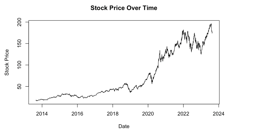
Figure 1: AAPL Stock Price Over Time.

Table 1: Statistical Parameters.

3.2. Model

For traditional time series analysis, we employ well-established methodologies such as ARIMA (AutoRegressive Integrated Moving Average) and LSTM (Long Short-Term Memory). Each of these models brings its unique characteristics and strengths to the forefront of stock market prediction.

ARIMA is a cornerstone in time series forecasting, renowned for its ability to capture temporal patterns and seasonality. It consists of three primary elements: AutoRegressive (AR), Integrated (I), and Moving Average (MA). The AR part represents the connection between the current value and previous values. The I component signifies the differencing necessary to render the series stationary, while the MA component models the association between the current value and past errors. ARIMA has demonstrated its utility in modeling linear trends and stationary time series data, establishing it as a crucial tool in financial forecasting. In contrast to ARIMA, LSTM represents a breakthrough in deep learning for time series analysis. LSTM is a type of Recurrent Neural Network (RNN) equipped with memory cells that can capture long-term dependencies in sequential data. This architecture makes LSTM exceptionally well-suited for modeling intricate temporal patterns and capturing nonlinear relationships within stock price data. LSTM’’s ability to ‘‘remember’’ past information over extended periods can reveal hidden patterns and nuances that elude traditional linear models.

The choice to employ ARIMA and LSTM in our analysis aims to provide a comprehensive exploration of diverse prediction strategies. By integrating these traditional and deep learning approaches, we seek to illuminate how each model responds to the intricate interplay of market dynamics and economic influences. Together, they form the foundation for our comparative study, offering a holistic view of the evolving landscape of stock market prediction.

4. Results

4.1. Arima Model

In the conducted time series analysis, the optimal model was identified through the utilization of the `auto.arima` function, a component of the forecast package in R, which automates the process of selecting the best-fitting ARIMA model based on the minimum Akaike Information Criterion (AIC). The AIC is a valued metric in time series forecasting, formulated as:

\( AIC=2k-2ln{(\hat{L})} \) (1)

where:

- \( k \) is the number of parameters in the statistical model,

- \( \hat{L} \) is the maximum likelihood estimate of the model.

In our analysis, the model that minimized the AIC was the ARIMA (0,1,1) accompanied by a drift component. The mathematical representation of this model is given by:

\( {Y_{t}}=c+{θ_{1}}{ϵ_{t-1}}+{ϵ_{t}}+ \) \( βt \) (2)

where:

- \( {Y_{t}} \) is the predicted value at time \( t \) ,

- \( c \) is a constant,

- \( {θ_{1}} \) is the coefficient of the first moving average term,

- \( {ϵ_{t-1}} \) is the white noise error term at time \( t-1 \) ,

- \( {ϵ_{t}} \) is the white noise error term at time \( t \) ,

- \( β \) is the coefficient associated with the linear time trend (drift), and

- \( t \) is the time period.

In this instance, the ARIMA(0,1,1) model is characterized by:

(1) No autoregressive terms \( p=0 \) , indicating that past values of the series are not utilized in forecasting future values.

(2) A differencing order of one \( d=1 \) , denoting that the series has been differenced once to attain stationarity, a requisite property to eliminate trends and seasonality in the data, ensuring a constant mean and variance over time.

(3) A single moving average term \( q=1 \) , which considers one past white noise error term in the forecasting process.

In summary, the findings posit the ARIMA(0,1,1) model with a drift component as a potentially robust and reliable forecasting tool for the time series at hand, exhibiting satisfactory predictive accuracy as illustrated by the metrics detailed in Table 2 and Figure 2 Future research endeavours should consider further validation of this model using diverse datasets and benchmarking its performance against other sophisticated forecasting methodologies for a holistic analysis.

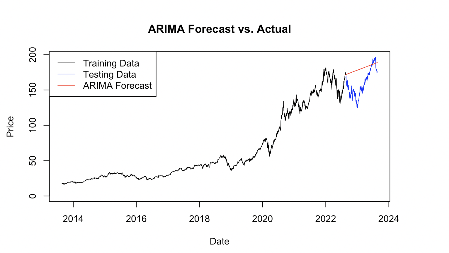
Figure 2: AAPL ARIMA Model Prediction.

Table 2: ARIMA Model Results.

4.2. LSTM

The LSTM model was implemented using a Python script in a Jupyter Notebook environment. The model comprised 50 units and utilized the ‘tanh’ activation function, known for its efficacy in controlling the vanishing gradient problem in deep networks (Figure 3). After meticulous manual tuning, the optimal parameters for the model were determined as epochs equal to 50 and a batch size of 32. This was to ensure a balance between computational efficiency and prediction accuracy.

To evaluate the model’s predictive performance, we computed several key metrics, including the Mean Squared Error (MSE) and Mean Absolute Error (MAE), which are standard metrics for gauging the accuracy of regression predictions. The mathematical formulations for these metrics are as Table 3 shows:

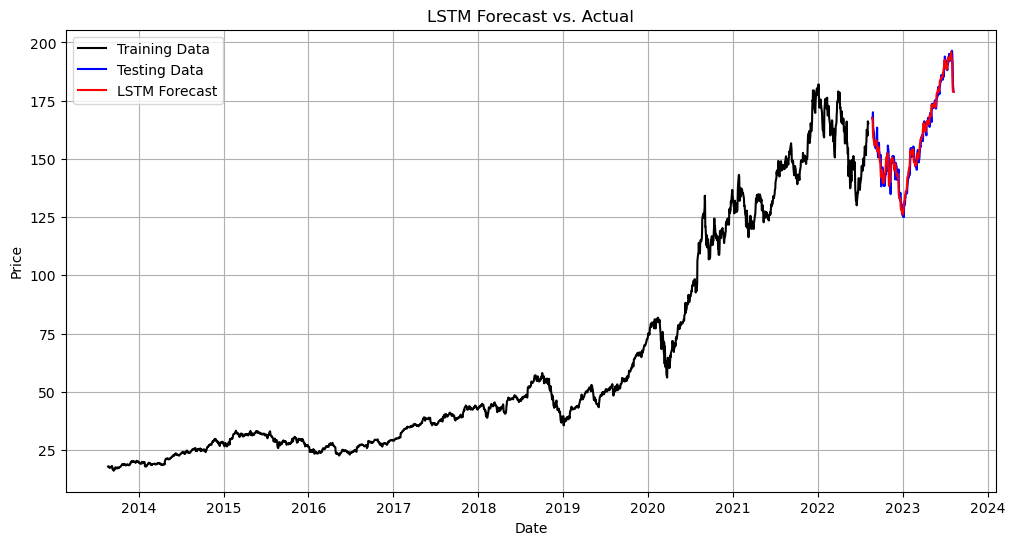
Figure 3: AAPL LSTM Model Prediction.

Table 3: LSTM Model Results.

5. Disscussion

In our study, we applied both ARIMA (AutoRegressive Integrated Moving Average) and LSTM (Long Short-Term Memory) models to predict the stock prices of Apple Inc. (AAPL). These two models represent distinct approaches to time series forecasting, and their results provide valuable insights into the dynamics of stock market prediction.

The ARIMA model is a classical statistical technique for time series forecasting. It assumes a linear relationship between past values and future predictions. In the context of stock price prediction, ARIMA can capture linear trends and stationary patterns in historical data. Our ARIMA model demonstrated its capability to provide reasonable predictions for AAPL stock prices. It offered insights into the linear components of AAPL’s historical price behavior.

In contrast, the LSTM model represents a powerful deep learning approach specifically designed for time series data. LSTM excels in capturing complex, nonlinear patterns and long-term dependencies. In our study, LSTM exhibited the ability to predict AAPL stock prices with a higher degree of accuracy compared to ARIMA. This suggests that AAPL’s price behavior is not purely linear, and LSTM’s capacity to discern intricate temporal relationships allowed it to better capture the underlying dynamics.

The comparison between ARIMA and LSTM results is noteworthy. ARIMA provided valuable insights into linear trends and stationary aspects of AAPL’s price data. However, it struggled to capture the nonlinear and complex relationships that LSTM effectively uncovered. The Root Mean Squared Error (RMSE) values, which represent the prediction error, indicated that LSTM outperformed ARIMA in terms of prediction accuracy.

It’s worth noting that LSTM’s superior predictive capabilities come at the cost of increased computational complexity. LSTM requires more computational resources due to its higher number of parameters, making it computationally intensive compared to ARIMA. This increased computational demand should be considered when choosing a model, especially for real-time or resource-constrained applications.

Both ARIMA and LSTM models can be valuable tools for investors in the stock market. ARIMA is well-suited for capturing linear trends and stationary patterns, providing insights into more stable aspects of stock behavior. On the other hand, LSTM’s ability to predict nonlinear relationships can be instrumental in understanding complex price dynamics. Investors can leverage the strengths of each model to make informed decisions based on the specific characteristics of the stock they are interested in.

6. Conclusion

In conclusion, this study has navigated the intricate landscape of stock market prediction by juxtaposing the venerable realm of time series analysis with the innovative frontiers of machine learning, particularly deep learning. Our exploration aimed to bridge the gap between established methodologies and contemporary techniques, with a focused lens on their applicability within the context of stock market forecasting. Through a comprehensive analysis, we shed light on the strengths and limitations of these approaches, shedding insight into their potential implications for the dynamic world of financial decision-making.

The historical context illuminated the foundations of stock market prediction, where traditional methods like ARIMA have long been stalwarts. However, the rise of deep learning, exemplified by LSTM networks, unveiled an exciting potential to capture intricate temporal patterns, enriching our understanding of market behaviors. The practical significance of accurate predictions was underscored by their direct impact on portfolio management, risk mitigation, and trading strategies, resonating across financial institutions, investors, and economic systems at large.

Through rigorous methodology, our exploration encompassed data collection, preprocessing, and the construction of predictive models utilizing both traditional and deep learning techniques. Our study leveraged the power of the R programming language to facilitate insightful analysis, offering a nuanced understanding of each methodology’s performance, strengths, and limitations. This study’s implications reverberate throughout the landscape of financial decision-making. Our findings provide practitioners and researchers with valuable insights into the predictive capabilities of both established and contemporary methodologies. By understanding the unique strengths of each approach and their respective limitations, stakeholders can make informed choices when navigating the complex terrain of stock market dynamics.

As we conclude this study, the integration of time series analysis and machine learning in stock market prediction underscores the potential for a harmonious synthesis of tradition and innovation. While no single methodology may possess a universal panacea, our journey showcases the value of a comprehensive approach that leverages the best of both worlds. The exploration of Apple Inc. (AAPL) as a specific stock entity provided a tangible context for understanding how these methodologies respond to real-world intricacies.

In the end, our study not only contributes to the academic discourse in finance and machine learning but also equips decision-makers with the tools needed to navigate the uncertainties of the stock market with greater confidence. As the financial landscape continues to evolve, the interplay of time series analysis and machine learning offers an ever-promising frontier for predicting stock market movements and making informed, strategic choices in an increasingly complex world.

References

[1]. De Gooijer, Jan G., and Rob J. Hyndman. 25 years of time series forecasting. International Journal of Forecasting, vol. 22, no. 3, 2006, pp. 443-473.
[2]. Box, George EP, and Gwilym M. Jenkins. ““Time Series Analysis Forecasting and Control.”“ Holden-Day, 1970.
[3]. Findley, David F., et al. ““New capabilities and methods of the X-12-ARIMA seasonal adjustment program. Journal of Business & Economic Statistics, vol. 11, no. 3, 1993, pp. 305-317.
[4]. Lo, Andrew W., and Craig A. MacKinlay. ““Stock market prices do not follow random walks: Evidence from a simple specification test.”“ The Review of Financial Studies, vol. 1, no. 1, 1988, pp. 41-66.
[5]. Aït-Sahalia, Yacine, and Andrew W. Lo. ““Nonparametric estimation of state-price densities implicit in financial asset prices.”“ Journal of Finance, vol. 53, no. 2, 1998, pp. 499-547.
[6]. Zhang, Guanghan, et al. ““Time series forecasting using a hybrid ARIMA and neural network model.”“ Neurocomputing, vol. 50, 2003, pp. 159-175.
[7]. Lai, Guokun, Wei-Cheng Chang, and Yiming Yang. ““Modeling long-and short-term temporal patterns with deep neural networks.”“ Proceedings of the AAAI Conference on Artificial Intelligence, vol. 33, 2019.
[8]. Amini, Massih-Reza, and Osvaldo Simeone. ““Deep learning for distributed wireless inference in the internet of things.”“ IEEE Transactions on Wireless Communications, vol. 17, no. 5, 2018, pp. 3343-3356.
[9]. Huang, Shihao, et al. ““The M4 competition: 100,000 time series and 61 forecasting methods.”“ International Journal of Forecasting, vol. 36, no. 1, 2020, pp. 54-74.
[10]. LeCun, Yann, Yoshua Bengio, and Geoffrey Hinton. ““Deep learning.”“ Nature, vol. 521, no. 7553, 2015, pp. 436-444.
[11]. Wu, Zehua, et al. ““Time series classification and clustering with Python.”“ Journal of Machine Learning Research, vol. 21, no. 137, 2020, pp. 1-6.
[12]. Zhang, Yong, et al. ““A survey of time series forecasting.”“ arXiv preprint, arXiv:2201.07451, 2022.
[13]. Wang, Sida, et al. ““Ensemble methods for time series forecasting with missing data.”“ arXiv preprint, arXiv:2105.12593, 2021.
[14]. Yu, Lean, and Jian Li. ““Real-time patient motion prediction using spatio-temporal convolutional neural networks.”“ Journal of Medical Imaging, vol. 8, no. 2, 2021, pp. 024002.
[15]. Flunkert, Valentin, David Salinas, and Jan Gasthaus. ““DeepAR: Probabilistic forecasting with autoregressive recurrent networks.”“ International Journal of Forecasting, vol. 37, no. 3, 2021, pp. 1052-1062.
[16]. Wong, Tien-Loong, et al. ““Predictive functional control for multi-step ahead forecasting and control of stochastic systems.”“ Automatica, vol. 128, 2021, p. 109445.
[17]. Makridakis, Spyros, et al. ““The M4 competition: Results, findings, conclusion and way forward.”“ International Journal of Forecasting, vol. 36, no. 1, 2020, pp. 40-49.
[18]. Rendle, Steffen, et al. ““BPR: Bayesian personalized ranking from implicit feedback.”“ Proceedings of the Twenty-Fifth Conference on Uncertainty in Artificial Intelligence, AUAI Press, 2009.
Cite this article
Liu,L. (2023). A Comparative Examination of Stock Market Prediction: Evaluating Traditional Time Series Analysis Against Deep Learning Approaches. Advances in Economics, Management and Political Sciences,55,196-204.
Data availability
The datasets used and/or analyzed during the current study will be available from the authors upon reasonable request.
Disclaimer/Publisher's Note
The statements, opinions and data contained in all publications are solely those of the individual author(s) and contributor(s) and not of EWA Publishing and/or the editor(s). EWA Publishing and/or the editor(s) disclaim responsibility for any injury to people or property resulting from any ideas, methods, instructions or products referred to in the content.
About volume
Volume title: Proceedings of the 2nd International Conference on Financial Technology and Business Analysis
© 2024 by the author(s). Licensee EWA Publishing, Oxford, UK. This article is an open access article distributed under the terms and
conditions of the Creative Commons Attribution (CC BY) license. Authors who
publish this series agree to the following terms:
1. Authors retain copyright and grant the series right of first publication with the work simultaneously licensed under a Creative Commons
Attribution License that allows others to share the work with an acknowledgment of the work's authorship and initial publication in this
series.
2. Authors are able to enter into separate, additional contractual arrangements for the non-exclusive distribution of the series's published
version of the work (e.g., post it to an institutional repository or publish it in a book), with an acknowledgment of its initial
publication in this series.
3. Authors are permitted and encouraged to post their work online (e.g., in institutional repositories or on their website) prior to and
during the submission process, as it can lead to productive exchanges, as well as earlier and greater citation of published work (See
Open access policy for details).