1. Introduction

House price prediction has always been an interesting area to do research on. There has been a lot of research done on this topic and new research keeps emerging these days. The decision on this topic was inspired by the recent shifts in house prices in California due to the pandemic. House prices had been dramatically surging and plunging in the last few months and it must be essential for consumers and investors to accurately estimate the actual value of a property. Thus, in the paper, the author decided to construct a model that can help people to estimate the real value of a house based on factors such as property characteristics and locations. The approach was inspired by Zestimate, which uses various variables and a neural network approach to provide an estimation of house value to consumers. According to the paper Zillow’s Estimates of Single-Family Housing Values, the prediction model could be able to produce an estimation within 10% of the actual transaction value [1].

2. Datasets and Variables

To discover the main factor that determines the house price, the author selected the dataset including 21,613 King County house prices with house characteristics from May 2014 to May 2015. Investigating the correlation between house values and house characteristics, the paper will be looking into each housing feature’s correlation with house market values [2].

Bedrooms: the number of bedrooms.

Bathrooms: the number of bathrooms, where 0.5 refers to bathrooms with no showers.

Sqftliving: the square footage of the house.

Sqrt-lot: the square footage of the land space.

Floors: the number of building floors.

Waterfront: 1 if the house has a waterfront view and 0 otherwise.

View: an index from 0 to 4. 0 indicates the worst view and 4 indicates the best view.

Condition: an index from 1 to 5 on the condition of the apartment.

Grade: an index from 1 to 13, where a score of 1-3 indicates the building is short of construction and design, 7 has an average level of construction and design, and 11-13 has a high-quality level of construction and design.

Sqftabove: the square footage of the house without counting the basement.

Sqftbasement: the square footage of the basement.

Yr-built: the year the house was built.

Yr-renovated: the year of the house’s last renovation.

Zipcode: the zip code of the house.

Sqftliving15: the living space size in 2015 (after innovation).

Sqftlot15: the land space area in 2015 (after innovation).

2.1. Descriptive Table

To perform further analysis of the data, since there are both continuous and quantitative data in the data set, it is essential to present the data in the form of a descriptive table to visualize the range of each variable. A descriptive table is also a great tool to examine if there exists any extreme outlier or abnormal variable value [3].

Table 1 presents a total of 21,612 pieces of housing information, indicating a large enough dataset to draw further conclusions on the relationship between house prices and other housing features. Removing one house with 33 bedrooms reduces potential extreme outlier bias since the median of the bedrooms is 3 with a standard deviation of 0.9. From the information, it is important to notice that the land space (sqftlot) has a large standard deviation of 41,421, with a minimum size of 520 and a maximum size of 1,651,359. With the most bathroom counts being 8, the standard deviation is 0.8 with a mean of 2.1. Finally, the mean value is 7.7 for grade and 3.4 for condition. Two numbers are close to the median value of the two features, which means that the data collected have included a fair amount of good and bad design, as well as houses in good and poor conditions. On the one hand, such information shows that the dataset includes a variety of house types. On the other hand, it also alerts people to the possibility that the effectiveness of the regression model would be downplayed by the presence of extreme outliers.

Table 1. King county house data (continue).

2.2. Housing Distribution

To better understand the distribution of the dataset, the paper plotted the houses by longitude and latitude. From the map shown in Figure 1, it can be clearly observed that the homes in the dataset are spread out across the King County.

2.3. Correlation Table

From Figure 2, it is important to notice that bathrooms, sqftliving, grade, sqftabove, and sqftliving15 have a relatively higher correlation with the price factor, therefore, it would be reasonable to focus on these factors in further analysis.

2.4. Plot Graph for Variables in the Base Model

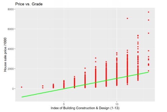
From Figure 3, there exists a strong and positive correlation between the house sales price and the square footage of the living space, as the line of best fit trends upwards and the data points follow the pattern. In addition, it is also important to notice that most data points are located on the left side of the graph and there are a few extreme outliers spread around the graph. For instance, there are three points located around 10,000 square footage of living space with prices around and above 7,000,000 dollars, which could cause potential bias in the regression results. As seen in Figure 4, there also exists a clear pattern of increase in the house price as the index of building construction design increases. Therefore, it is reasonable to conclude that there is a positive correlation between the grade and the house selling price.

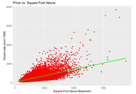
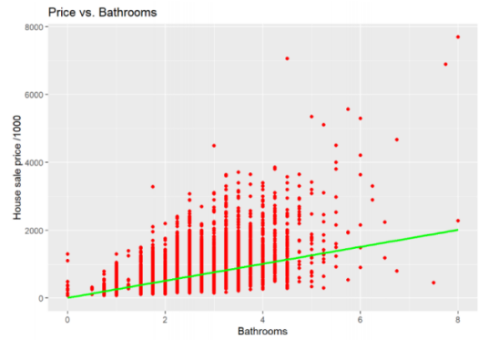
According to Figure 5, there exists a positive correlation between the house market value and the square footage above the basement. Like the correlation graph between price and square footage of living space shown in Figure 3, it is important to pay attention to the three outliers located around 8500 square feet with house price over 7,000,000 dollars. Plotting bathroom variables as shown in Figure 6 results in a positive correlation between the house price and the number of bathrooms in the building.

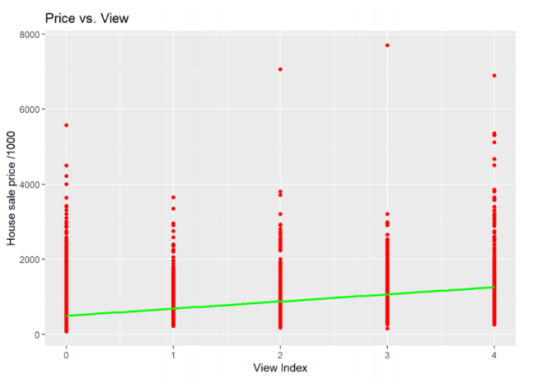
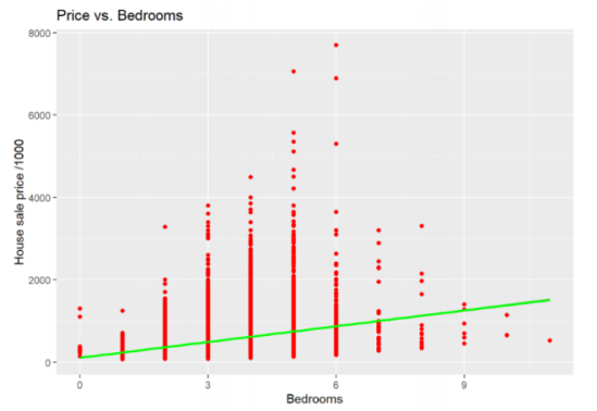
As seen in Figure 7, there exists a positive correlation between the view index and the house price. However, this correlation is more gradual compared to the previous one. According to Figure 8, there is a positive correlation between the number of bedrooms and the house sales price.

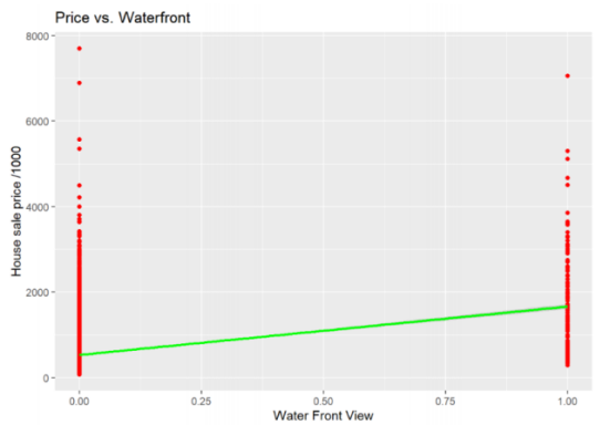
Finally, as shown in Figure 9, for the binary waterfront variable, houses with a waterfront view have a relatively higher price than those without a waterfront view.

3. Model Selection

After observing all the variables of interest that have a positive correlation with the house price, it would be reasonable to conduct further analysis. The model used to analyze the correlation between the independent variable (house price) and the dependent variables will be linear regression.

\( {Y_{i}}= {β_{0}}+ {β_{1}}{X_{i}} \) (1)

The final model of this research includes multiple independent variables to predict the dependent price variable. Thus, a multiple regression model will be introduced to explain a more accurate estimation [6].

\( Y= {β_{0}}+ {β_{1}}{X_{1}}+ {β_{2}}{X_{2}}+…+{β_{i}}{X_{i}} \) (2)

4. Result and Analysis

4.1. First Regression Analysis

The first regression table (Table 2) shows the correlation between the independent variables and the house price.

Table 2. First regression table.

4.1.1. Regression 1

Holding other variables the same, one additional square foot increase in the living space would increase the house value by 184.528 dollars. One additional grade index would increase the house value by 98,638.39 dollars.

4.1.2. Regression 2

Holding other variables the same, one additional square foot increase in the living space would increase the house value by 234.822 dollars. One additional grade index would increase the house value by 110,076.6 dollars. One additional square foot of the building apart from the basement would decrease the house value by 77.762 dollars.

4.1.3. Regression 3

Holding other variables the same, one additional square foot increase in the living space would increase the house value by 252.69 dollars. One additional grade index would increase the house value by 115,149.2 dollars. One additional square foot of the building apart from the basement would decrease the house value by 76.931 dollars. One additional bathroom count would decrease the house value by 37,098.19 dollars.

4.1.4. Regression 4

Holding other variables the same, one additional square foot increase in the living space would increase the house value by 209.106 dollars. One additional grade index would increase the house value by 104,006.9 dollars. One additional square foot of the building apart from the basement would decrease the house value by 41.49 dollars. One additional bathroom count would decrease the house value by 29,907.69 dollars. One additional view index would increase the house value by 92,223.54 dollars.

4.1.5. Regression 5

Holding other variables the same, one additional square foot increase in the living space would increase the house value by 233.108 dollars. One additional grade index would increase the house value by 97,802 dollars. One additional square foot of the building apart from the basement would decrease the house value by 44.962 dollars. One additional bathroom count would decrease the house value by 19,956.71 dollars. One additional view index would increase the house value by 88,606.23 dollars. One more bathroom in the house would decrease the house price by 35,297.97 dollars.

4.1.6. Regression 6

Holding other variables the same, one additional square foot increase in the living space would increase the house value by 233.774 dollars. One additional grade index would increase the house value by 100,119.9 dollars. One additional square foot of the building apart from the basement would decrease the house value by 49.574 dollars. One additional bathroom count would decrease the house value by 20,574.48 dollars. One additional view index would increase the house value by 61,595.69 dollars. One more bathroom in the house would decrease the house price by 32,218.98 dollars. A house with a waterfront view would raise the house value by 585,638 dollars. It is important to note that all the variables included in the first regression table are statistically significant, which means that it is reasonable to reject the null hypothesis and conclude that there is a strongly positive or negative correlation between the dependent variables and the price. Of all the regression models, however, it is important to note that the optimal R2 value is only 0.596, meaning that only 59.6 percent of the variation in the dependent variable can be explained by the independent variables. As a result, the author decided to further develop the 6th regression model since it explains the most variance in price.

4.2. Second Regression Analysis

For the second regression table (Table 3), the author has replaced the variables of sqftabove, bedrooms, and bathrooms since they have a limited impact on the R2. The paper added sqftliving15 and yr-built. In addition, it can be clearly observed from Figure 1 that houses located in the northwest generally have a higher price. According to the paper House Prices and Relative Location, the walking distance to key locations such as parks, schools, and hospitals has a high explanatory power on house prices, thus it would be reasonable to consider latitude and longitude to the regression analysis [7,8].

Table 3. Second regression table.

4.2.1. Regression 1

Holding other variables the same, one additional square footage of living space would increase the house price by 164.751 dollars. One more grade index would increase the house market value by 93,850.1 dollars. One additional square footage of living in 2015 would raise the house price by 3.447 dollars. One more view index would increase the house price by 70,447.32 dollars. A house that has a waterfront view would be worth 590,653.6 dollars more than those that do not.

4.2.2. Regression 2

Holding other variables the same, one additional square footage of living space would increase the house price by 159.189 dollars. One more grade index would increase the house market value by 133,157.4 dollars. One additional square footage of living in 2015 would raise the house price by 14.039 dollars. One more view index would increase the house price by 47,477.68 dollars. A house that has a waterfront view would be worth 597,910.4 dollars more than those that do not. One more later the house was built would decrease the house value by 3,284 dollars.

4.2.3. Regression 3

Holding other variables the same, one additional square footage of living space would increase the house price by 166.488 dollars. One more grade index would increase the house market value by 108,952.9 dollars. One additional square footage of living in 2015 would raise the house price by 24.641 dollars. One more view index would increase the house price by 50,664.2 dollars. A house that has a waterfront view would be worth 611,701.9 dollars more than those that do not. One more later the house was built would decrease the house value by 2395.714 dollars. One more degree increase in latitude would increase the house value by 557,820.6 dollars. One more degree increase in longitude would decrease the house price by 108,761.3 dollars.

The impact of coordinates can be explained in Figure 1. It can be clearly observed that houses to the northwest are generally more expensive than the surrendering area.

4.2.4. Regression 4

For this last regression, the author has taken the log of price. Doing so would reduce the lack of generalization of the dependent variable, normalizing it so that it would be easier to draw a correlation. The adjusted R2 for this regression is 0.753, which means that 75.3% of the variance in price has been explained by this regression model. With all the independent variables being statistically significant, this paper decided to accept it as the final regression model.

5. Conclusion

The Final Model of King County House Price Prediction:

log(price)= -54.527 + (0.0002)sqftliving + (0.174)grade + (0.0001)sqftliving15 + (0.061)view + (0.39)waterfront - (0.003)yr - built + (1.354)latitude - (0.058)longitude

The model means that while holding other variables constant, one additional square footage of living space would increase the house price by 0.02%. One additional grade index would increase the house price by 17.4%. One more square footage of living space in 2015 would increase the house value by 0.01%. One additional view index would increase the house price by 6.1%. A house with a waterfront view would raise the property value by 39%. One year increase in the year built would decrease the house price by 0.3%. One degree increase in latitude would raise the house price by 135.4% (1 degree latitude ~ 69 miles). One degree increase in longitude would decrease the house value by 5.8% (1 degree longitude ~ 54.6 miles). According to the regression result, it is surprising to see how the property location can have such a huge impact on the house market value. One degree latitude increase would raise the property value by 135.4%, which means that one additional mile to the north would raise the house price by 1.96%. The waterfront variable is one of the most significant variables economically. Having a waterfront view makes a 39% difference in the house value. Grade is the second economically significant factor; each level makes a 17.4% difference. Since there are 13 levels of grade, the difference between a low grade and a high grade can easily cause a larger effect on the price than the waterfront does.

However, it is important to realize that the adjusted R2 for the final model is 0.753, meaning that 75.3% of the variation of the house price is explained by the model and 24.7% of the price variations are undermined by the variables. This is caused by the omitted variable bias, meaning that some confounding variables are not included in the regression model. As a result, the prediction made by this model may not be exactly accurate and should be used only for basic reference but not for detailed analysis. Most importantly, the external validity of the house price prediction model is low since the dataset only included the housing data in King County, WA. If the prediction of this model is applied to other states or cities, the result may not be accurate due to economic, cultural, and geographic factors. For instance, if the model is to predict the house price for an inland city in Texas, the results will not be as accurate since there would be very few houses with a waterfront view.

References

[1]. Hollas, D., et al.: Zillow’s Estimates of Single-Family Housing Values: Semantic Scholar. Zillow’s Estimates of Single-Family Housing Values. Semantic Scholar. (1970). https://www.semanticscholar.org/paper/Zillow-%E2%80%99-s-Estimates-of-Single-Family-Housing-Hollas-Rutherford/ca1a7e03f08380dce18ff5f766f1bd4301a42201#paper-header.
[2]. Harlfoxem. House Sales in King County, USA. Kaggle. (2016). https://www.kaggle.com/datasets/harlfoxem/housesalesprediction.
[3]. Spriestersbach, A., et al.: Descriptive Statistics: The Specification of Statistical Measures and Their Presentation in Tables and Graphs. Part 7 of a Series on Evaluation of Scientific Publications. Deutsches Arzteblatt International, Deutscher Arzte Verlag. (2009). https://www.ncbi.nlm.nih.gov/pmc/articles/PMC2770212/.
[4]. Ambarish, B.: Tutorial Housesales Kingcounty EDA&Modelling. Kaggle. (2018). https://www.kaggle.com/code/ambarish/tutorial-housesales-kingcounty-eda-modelling/report.
[5]. Dhakre, A.: EDA: Linear Regression: K-Fold CV: ADJ R2=0.87. Kaggle. (2017). https://www.kaggle.com/code/amitdhakre13/eda-linear-regression-k-fold-cv-adj-r2-0-87.
[6]. Marill, K. A.: Advanced Statistics: Linear Regression, PART II ... - Wiley Online Library. Wiley Online Library. https://onlinelibrary.wiley.com/doi/pdf/10.1197/j.aem.2003.09.006.
[7]. Heyman, A. V., Sommervoll, D. E.: House Prices and Relative Location. ScienceDirect. (2019). https://www.sciencedirect.com/science/article/pii/S0264275118312241.
[8]. Rivas, R., Patil, D., Hristidis, V. et al.: The impact of colleges and hospitals to local real estate markets. J Big Data 6, 7 (2019). https://doi.org/10.1186/s40537-019-0174-7.
Cite this article
Cui,Z. (2023). House Price Prediction with Big Data. Advances in Economics, Management and Political Sciences,6,85-93.
Data availability
The datasets used and/or analyzed during the current study will be available from the authors upon reasonable request.
Disclaimer/Publisher's Note
The statements, opinions and data contained in all publications are solely those of the individual author(s) and contributor(s) and not of EWA Publishing and/or the editor(s). EWA Publishing and/or the editor(s) disclaim responsibility for any injury to people or property resulting from any ideas, methods, instructions or products referred to in the content.
About volume
Volume title: Proceedings of the 2022 International Conference on Financial Technology and Business Analysis (ICFTBA 2022), Part 2
© 2024 by the author(s). Licensee EWA Publishing, Oxford, UK. This article is an open access article distributed under the terms and
conditions of the Creative Commons Attribution (CC BY) license. Authors who
publish this series agree to the following terms:
1. Authors retain copyright and grant the series right of first publication with the work simultaneously licensed under a Creative Commons
Attribution License that allows others to share the work with an acknowledgment of the work's authorship and initial publication in this
series.
2. Authors are able to enter into separate, additional contractual arrangements for the non-exclusive distribution of the series's published
version of the work (e.g., post it to an institutional repository or publish it in a book), with an acknowledgment of its initial
publication in this series.
3. Authors are permitted and encouraged to post their work online (e.g., in institutional repositories or on their website) prior to and
during the submission process, as it can lead to productive exchanges, as well as earlier and greater citation of published work (See
Open access policy for details).