1.Introduction

Stocks are one of the main forms of securities. It is a joint-stock company raising capital issued to the investors' share certificates on behalf of its holders (i.e., shareholders) on the joint-stock company's ownership [1]. The purchase of shares is also to buy a part of the enterprise business and can be the common growth and development of the enterprise. With the gradual improvement and development of the world economy, the stock market has gradually become the most widely traded market today [2].

The ARIMA model, known as the Autoregressive Moving Average Model with Differences, is a well-known time series forecasting method proposed by Box and Jenkins in the early 1970s, so it is also known as the box-Jenkins model. The ARIMA model is built by transforming a non-stationary time series into a stationary time series and then regressing the dependent variable only on its lagged value and the stochastic error term's present and lagged values [3]. The model was developed by regression [3]. Where ARIMA (p, d, q) is called the differential autoregressive moving average model, AR is autoregressive, p is the autoregressive term; MA is the moving average, q is the number of moving average terms, and d is the number of differentials made when the time series becomes smooth. This model is one of the most popular time series analysis models in recent years, which improves the existing time series analysis models to make the model simpler to apply [4]. ARIMA model is also widely used in stock price forecasting, house price forecasting and value trend forecasting due to its good operability and high accuracy [5, 6].In this article, python is chosen as the language environment and machine learning and mathematical regression models are used to implement the ARIMA model to predict the closing price of a stock, and the data comparison is used to study whether the original data will significantly affect the prediction results of the ARIMA model.

This paper presents the realization process and conclusions of the topic in four aspects: the first part is a background introduction, the second part is the experimental process and results, the third part is a discussion based on the results, and the fourth part is a conclusion statement.

2.Experimental procedure

2.1.Continuous data

2.1.1.Data preprocessing

Firstly, the raw data needs to be divided into two groups, i.e. the training group and the test group. The data in the training group is trained using the ARIMA model, and the predictions obtained from it are compared with the data in the test group to determine if the predictions obtained from the training data are approximately the same as those obtained from the test data. The comparison results can be used to analyse how well the model fits the data.

In this section, the stock closing prices of a Chinese bank for the years 2005-2017 are selected as the training data and the stock closing prices for the years 2018-2021 are chosen as the test data. As new training data, the closing prices are resampled and averaged on a weekly basis to fill in possible gaps in the original data and to give it continuity.

2.1.2.ADF test

In the data model analysis and prediction before, first of all, to determine whether the data is smooth. According to the understanding of the ARIMA model can be known only smooth data can be used ARIMA model for prediction and analysis, so this step is intended to determine whether data is smooth data. In this part of the detection of whether the data is smooth method is to data ADF test, that is, to carry out the unit root test. ADF test is based on the presence of a unit root in the data to determine whether the data is in a smooth state [7]; if the data does not exist in the unit root, that is, the p-value is less than 0.5, the ADF value is less than 0.5, then it means that the data is smooth data, can be used for subsequent experiments and analysis. If it is not smooth, then the data needs to be differenced until it meets the criteria for smooth data.

ADF test formula:

\( ADF=({Y_{t}}-{Y_{t-1}})-δ{Y_{t-1}} \)(1)

ADF test results are showed in Figure 1.

Figure 1: Plot of first-order difference results

Table 1: First-order differential ADF values

As seen from Figure 1 and Table 1, the overall range of fluctuations in the data is relatively smooth, although some of the data fluctuate considerably. And it can be seen that the ADF value is less than the critical value at 10%, 5% and 1%, indicating that the data have reached a smooth state after the first-order differencing.

2.1.3.Determination of model parameters

Based on the autocorrelation and partial autocorrelation plot observations coupled with the AIC criterion, it can be determined that the model parameters at this point should be 2, 0, 0. Therefore, the model parameters are brought into the ARIMA model, predictions are made for the last 400 pieces of data, and the prediction result plots are compared to the original data for the previous four hundred pieces.

The AIC information criterion, Akaike information criterion, is a measure of the goodness of fit of a statistical model, as it was created and developed by the Japanese statistician Hiroji Akaike. It is based on the concept of entropy, which weighs the complexity of the estimated model against the goodness of fit of this model to the data [8]. In general, the smaller the AIC value, the better the model.

Formula for the AIC test:

\( AIC=-2ln{(L)+2K} \)(2)

BIC was developed by Gideon E. Schwarz, who applied Bayesian parameters to the criterion. It is similar to the Akaike Information Criterion (AIC), but BIC is more focused on dependence. BIC has a more significant penalty term than AIC [9].

Formula for the BIC test:

\( BIC=-2ln{(L)+ln{(n)*K}} \)(3)

However, to simplify the experiment, this part used the means of ACF and pace to determine the model parameters. The trailing and truncated nodes are used as the values of p and q in the ACF and PACF tests [10].

The Chart of ACF results is shown in Figure 2.

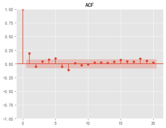
Figure 2: Chart of ACF results

PACF results are shown in Figure 3.

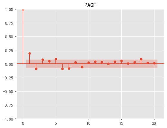
Figure 3: Chart of PACF results

The ACF detection plot shows that the data shows a truncated state after 1, so the q value is chosen here as 1. The PACF detection plot shows that the data shows a truncated state after 1, so the value of 1 is chosen here as the p-value. At the same time, as the data are differentiated once to obtain smooth data, the d in the model parameters is chosen to take the value of 1 [11].

2.1.4.Comparison of results

To facilitate the observation of the degree of a model fitting and accurate analysis of the prediction results, this part of the model predicted results in the form of a trend curve, with the original data of the stock on a chart for comparison, which not only facilitates the intuitive observation of the effect of model fitting but also easier to analyse the accuracy of the model prediction.

The results of Comparison are shown in Figure 4.

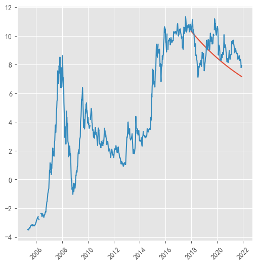
Figure 4: Results Comparison Chart

As can be seen from the figure, the overall fit of the model is better, and the trend curve of its prediction results is also basically similar to the trend of its actual data, so this set of data fits the ARIMA model better, and the predicted data are relatively accurate.

2.2.Discontinuous data

2.2.1.Data preprocessing

In this experiment, stock data for the same bank is selected for the period from 2020 to May 2023, and there are some data gaps in this set of data due to the fact that the interface for obtaining these stock data has been updated and some of the data has not been synchronized with the original interface. Different from the previous set of experiments, this data set is not predicted using the average weekly closing price but directly using the daily closing price, which may result in unfillable data gaps in the data. Therefore, this is a discontinuous data set.

In this step, this study splits the data into a training and a test group, with the first 60% of the data serving as the prediction group and the last 40% as the measurement group to test the model’s fit.

2.2.2.ADF test

This section performs a smoothness test on the test data as in the first set of experiments, and only if the data reaches a smooth state can it be used by the ARIMA model.

ADF test results:

Table 2: Six-order differential ADF values

Here it took six differencing runs to get smooth data with a p-value infinitely close to 0 and an ADF mean less than the 10% threshold. Here it may be since the original data is discontinuous, and hence it is very non-smooth data, to make it smooth data, multiple differencing has to be done. However, the difference between the data after six differencing and the original data becomes very large, so the subsequent experimental data may deviate from the original data resulting in a poor model fit.

2.2.3.Determination of model parameters

This part still uses the intuitive selection of model parameters by plotting ACF and PACF diagrams.

ACF results are showed in Figure 5:

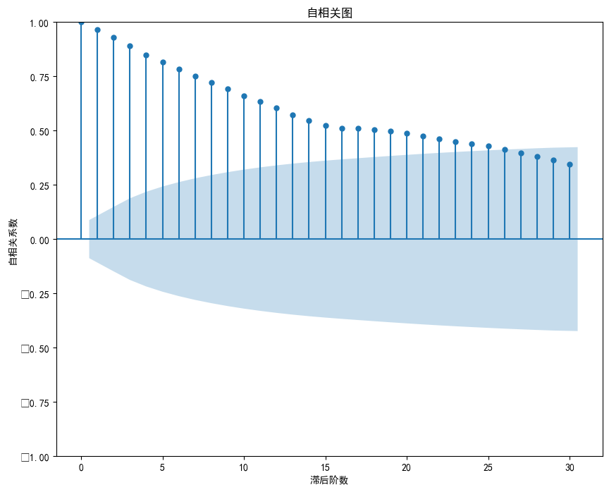
Figure 5: Chart of ACF results

It trails very far back in the ACF plot, so the q-value has to be chosen to be around 25, but this also means that it has poor predictive power and will be more biased in the subsequent fitting.

Chart of PACF results is shown in Figure 6:

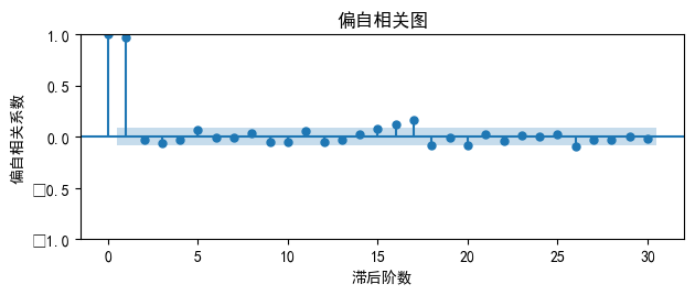
Figure 6: Chart of ACF results

In the PACF, it can be seen that after the first node, there is a truncated tail, so in this section, it can be determined that the value of p is chosen as 1. Since the data is differenced six times during the ADF test, the value of d is 6.

2.2.4.Comparison of results

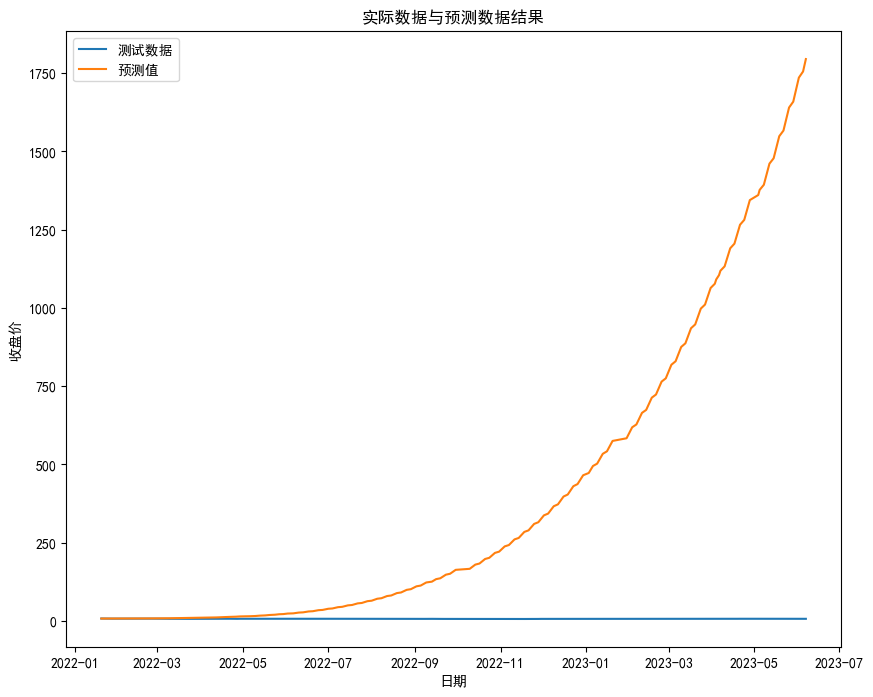
Figure 7: Results Comparison Chart

The predicted results and test data are put on a graph for observation. In Figure 7, the vertical axis represents the predicted values, the horizontal axis represents the date, the orange curve represents the predicted values, and the blue curve represents the test data. It can be seen that the predicted results are not in line with the actual results, and the difference between the two is very large. Therefore, it can be guessed that this result is because the original data is extremely unstable, and the multiple differencing has caused serious data loss, which in turn affects the prediction results and the fitting of the model.

3.Discussion

From the results of the above two experimental groups, it can be seen that in the first set of experiments, that is, when the original data is continuous, the ARIMA model fits the data better. The predicted trend is consistent with the trend of the test data, which proves that the prediction is also good. However, in the second set of experiments, the original data is discontinuous, and it can be seen that the training data requires at least 6 differentials to achieve smooth data, which in turn leads to more data loss, leading to severe deviation between the predicted data and the test data, making the model unable to fit the data. Through the analysis of the results, it can be speculated that the reason for the huge difference in results is more related to the integrity and smoothness of the original data, and the data with more missing data need to be filled in to use the ARIMA model for prediction. Deriving the initial data from this may directly affect the degree of fit of the ARIMA model.

4.Conclusion

The experimental study and the discussion of the results show that the experimental group with more data missing in the initial data obtained poor prediction results and showed a large deviation from the test data. On the other hand, the experimental group without a lot of missing data, performed well. Through the comparison and discussion of the results of the two experimental groups, it can be concluded that the data coherence of the original data has a significant impact on the prediction results of the ARIMA model and that the ARIMA model cannot be applied to a certain extent to the prediction of the original data with a large number of missing data. Although the comparison of the two experimental groups can get clearer experimental results and conclusions, this article still has the problem of insufficient experimental volume, and the experimental data come from the stock data website, which lacks the innovativeness of the data. Because of the problems in the article, it can be improved by increasing the number of experimental groups and the amount of data in each experimental group in the subsequent research. At the same time, in the future research process, we can also add a group of experiments to predict the future price of stocks and wait for the real price of stocks in the future and then compare with the prediction results to increase the authenticity and operability of the ARIMA model in the use of more consistent data prediction, so that the ARIMA model is used in the prediction of daily life. Based on the conclusions of this study, the research on data prediction using time-series models should be developed or explored in the subsequent development process to make more accurate predictions for non-coherent data with many data gaps. Most of the data in nature cannot have good coherence, so this may be an important future research direction.

References

[1]. King, B. F. (1966). Market and industry factors in stock price behavior. the Journal of Business, 39(1), 139-190.
[2]. Lucas, D. J., & McDonald, R. L. (1990). Equity issues and stock price dynamics. The journal of finance, 45(4), 1019-1043.
[3]. Shumway, R. H., Stoffer, D. S., Shumway, R. H., & Stoffer, D. S. (2017). ARIMA models. Time series analysis and its applications: with R examples, pp.75-163.
[4]. Ho, S. L., & Xie, M. (1998). The use of ARIMA models for reliability forecasting and analysis. Computers & industrial engineering, 35(1-2), 213-216.
[5]. Ariyo, A. A., Adewumi, A. O., & Ayo, C. K. (2014, March). Stock price prediction using the ARIMA model. In 2014 UKSim-AMSS 16th international conference on computer modelling and simulation, IEEE, pp. 106-112.
[6]. Mondal, P., Shit, L., & Goswami, S. (2014). Study of effectiveness of time series modeling (ARIMA) in forecasting stock prices. International Journal of Computer Science, Engineering and Applications, 4(2), 13.
[7]. Lopez, J. H. (1997). The power of the ADF test. Economics Letters, 57(1), 5-10.
[8]. Bozdogan, H. (1987). Model selection and Akaike's information criterion (AIC): The general theory and its analytical extensions. Psychometrika, 52(3), 345-370.
[9]. Vrieze, S. I. (2012). Model selection and psychological theory: a discussion of the differences between the Akaike information criterion (AIC) and the Bayesian information criterion (BIC). Psychological methods, 17(2), 228.
[10]. Demir, V., Zontul, M., & Yelmen, I. (2020, September). Drug sales prediction with ACF and PACF supported ARIMA method. In 2020 5th International Conference on Computer Science and Engineering (UBMK), IEEE, pp. 243-247.
[11]. Piccolo, D. (1990). A distance measure for classifying ARIMA models. Journal of time series analysis, 11(2), 153-164.
Cite this article
Yan,Y. (2024). Explore the Impact of Initial Data Coherence on ARIMA Model Prediction Based on Python. Advances in Economics, Management and Political Sciences,71,34-41.
Data availability
The datasets used and/or analyzed during the current study will be available from the authors upon reasonable request.
Disclaimer/Publisher's Note
The statements, opinions and data contained in all publications are solely those of the individual author(s) and contributor(s) and not of EWA Publishing and/or the editor(s). EWA Publishing and/or the editor(s) disclaim responsibility for any injury to people or property resulting from any ideas, methods, instructions or products referred to in the content.
About volume
Volume title: Proceedings of the 3rd International Conference on Business and Policy Studies
© 2024 by the author(s). Licensee EWA Publishing, Oxford, UK. This article is an open access article distributed under the terms and
conditions of the Creative Commons Attribution (CC BY) license. Authors who
publish this series agree to the following terms:
1. Authors retain copyright and grant the series right of first publication with the work simultaneously licensed under a Creative Commons
Attribution License that allows others to share the work with an acknowledgment of the work's authorship and initial publication in this
series.
2. Authors are able to enter into separate, additional contractual arrangements for the non-exclusive distribution of the series's published
version of the work (e.g., post it to an institutional repository or publish it in a book), with an acknowledgment of its initial
publication in this series.
3. Authors are permitted and encouraged to post their work online (e.g., in institutional repositories or on their website) prior to and
during the submission process, as it can lead to productive exchanges, as well as earlier and greater citation of published work (See
Open access policy for details).