1. Introduction

In recent years, the U.S. construction industry has experienced sluggish growth and slow adoption of new technologies [1]. In order to promote the growth of the construction industry and add value to construction firms, research on the impact of financial factors is essential to promote business development.

Currently, there are the following ideas to study the increase of enterprise value in the construction industry: study the increase of organizational capital to increase enterprise value, such as leadership, alignment of strategic goals, organizational design, and other factors. This approach determines enterprise value through modeling and qualitative analysis [2]. Constructing enterprise value through growth option modeling is based on the need for more traditional net present value to correctly capture intelligent and innovative firms' growth potential and management flexibility value. This approach determines whether the sub-projects of the enterprise are profitable and economically valuable by building a mathematical model and then by the size of the investment value [3]. Creating corporate value through non-financial factors, including human capital and human resources, are playing an increasingly important role based on the new economic era and knowledge economy. Repeating a one-way ANOVA, this method determines whether certain factors have a significant influence effect [4]. Through EVA (Economic Value Added), economic, accounting, and market factors are combined to comprehensively evaluate the value of a company taking into account accounting risks. This idea determines the enterprise value by building a neural network model [5].

Although these values are innovative and in line with the current trend towards a knowledge-based society and an innovation economy. However, these values are difficult to define and produce measurements under different criteria. The qualitative approach used to study organizational capital does not allow for a specific measurement of intangible capital, limiting this theory's operationalization and needing more specific data and statistical support. The growth option theory only establishes a mathematical model not operationalized with actual company data and needs real-world empirical support. The human resource theory only measures whether certain factors are significant or not and does not consider which factors are more influential on firm value, which factors need to be paid more attention to, and how much a change in a particular factor will bring about a specific amount of change in firm value.

In order to have a definite value for the value and its influencing factors, this study uses financial data from the stock market in wall street journal, this data is objectively standardized and operational. Selecting data from the stock market is close to the economic reality of the construction industry and makes the model rich in practical data support. Regression analysis establishes a linear relationship between firm value and financial data, such as debt ratio. This approach considers significance and utilizes variables such as correlation and regression coefficients to determine which factors are more influential, making the model more prosperous and instructive. It also utilizes dependent variables such as EV/EBITDA to remove the effects of the size of the enterprise value itself.

The study will then narrate the basic notion, and then the linear equation model will be explicitly analyzed and discussed based on the model to get the pattern. Finally, the conclusion is obtained.

2. Basic Notion

2.1. Regression Analysis Methods

Regression analysis is a statistical method of analyzing data to understand whether there is a correlation between two or more variables, the direction and strength of the correlation, and to develop mathematical models to look at specific variables to predict the variables of interest to the researcher. Regression analysis is a statistical technique that facilitates the comprehension of the extent of variation in the dependent variable when there is a singular alteration in the independent variable.

Regression analysis uses the least squares operation, and the following prerequisites need to be fulfilled when using this method: 1. The data needs to satisfy a normal distribution, and 2. The errors have the same variance for a given explanatory variable [6]. The formula for the least squares method is as follows:

\( y={β_{0}}+{β_{1}}x+ε \) (1)

where \( {β_{0}} \) , \( {β_{1}} \) is a non-random but unobservable parameter

x is a non-random and observable general variable

\( ε \) is an unobservable random variable, random error, or noise

y is an observable random variable

The best linear unbiased estimation formula for \( {β_{0}}{ and β_{1}} \) is as follows:

\( {β_{1}}=\frac{\sum {x_{i}}{y_{1}}-\frac{1}{n}\sum {x_{i}}\sum {y_{i}}}{\sum x_{i}^{2}-\frac{1}{n}{(\sum {x_{i}})^{2}}}, { β_{0}}=-{β_{1}} \) (2)

2.2. EV/EBITDA

The advantages of utilizing market share price valuation are that it is simple, intuitive and the market easily accepts the valuation results. Calculation using the fair asset value of the enterprise. The data comes from the open market, the calculation process is simple, the human influence factors are small, and it is easy to get the expected results [7].

The prerequisites for utilizing this method of valuation are the following two: 1. other listed companies in the same industry can be used as comparison objects for the assessed companies 2. there exists a sufficiently developed and active capital market and securities exchange market, and the market can correctly price the shares of these companies. As the most developed market in the world, the U.S. capital market has many listed companies in the construction industry that can be used as comparables for the target companies. Utilizing this method is fulfilling the prerequisites [7].

The specific formula for EV/EBITDA is as follows:

\( \frac{EV}{EBITDA}=\frac{Enterprise Value}{Earnings Before Interest, Taxes, Depreciation and Amortization} \) (3)

The implication behind this approach is that if assessing the value of a company, the researcher needs to consider not only its market value but also the liabilities assumed by the company. One notable benefit of this methodology lies in its capacity to facilitate the comparison of profitability across other organizations, despite disparities in their capital structures, tax rates, and policies regarding depreciation and amortization [8], and it also eliminates the effects of accounting and tax policies [9], allowing companies in different regions of the United States to compare values together. The disadvantage is that the valuation will be biased when there are more businesses [7]. However, the impact of this drawback is greatly minimized by the fact that this study focuses on studying construction firms with businesses limited to the construction industry.

2.3. Net Profit Margin

The net profit margin is a financial metric that quantifies the proportion of sales revenue that remains after subtracting all expenses and charges, including interest, taxes, and preferred stock dividends [10]. The formula used to calculate the net profit margin is as follows:

\( Net Profit Margin=\frac{R-COGS-E-I-T}{R}×100\%=\frac{Net Income}{R}×100\% \) (4)

R is Revenue.

COGS is The Cost of Goods Sold.

E is Operating and other costs.

I is Interest.

T is Tax.

This metric encompasses various operational aspects of the company, including total revenues, supplementary sales sources, cost of goods sold, other operating expenses, interest expense on debt, investment income, secondary operating income, and exceptional payments for atypical events like litigation and taxes.

The net profit margin is widely regarded as a crucial metric for assessing a company's profitability. The metric under consideration pertains to the proportion of a company's or business unit's net profit in relation to its revenue. The net profit margin is typically represented as a percentage. This metric demonstrates the profitability achieved per unit of sales revenue, accounting for all relevant business expenses incurred in generating those revenues. A greater margin indicates that a larger proportion of every dollar earned from sales is retained as profit.

2.4. Gross Profit Margin

The gross margin is a financial metric that quantifies the proportion of revenue that a company retains after deducting the cost of goods sold [10]. The equation used to compute gross margin is as follows:

\( Gross Profit Margin=\frac{Net sales-COGS}{Net sales}×100 \) \( \% \) (5)

COGS means the same as above

A company's gross margin indicates how much profit the company makes after taking into account the direct costs associated with conducting business. In brief, this metric provides an assessment of the company's ability to effectively translate sales into financial gain, denoted as revenue minus the expenses associated with the production of goods, encompassing labor and materials.

3. Model Analysis

3.1. Data Collection

In this study, the financial data of 34 U.S. listed construction companies in March 30, 2023, including EV/EBITDA, net profit margin, and gross profit margin, are selected from wall street journal. And the net profit margin and gross profit margin of each of these 34 companies are screened in two groups to compare the analysis results of different ranges of data.

Here are the data sets and what they represent:

• NPM1: Net Profit Margin value of the 34 companies with net profit margins between -5% and 5%

• NPMEBITDA1: EV/EBITDA value for the company represented by NPM1

• NPM2: Net Profit Margin value of the 34 companies with net profit margins between -6% and 10%

• NPMEBITDA2: EV/EBITDA value of the firms represented by NPM2

• GPM1: Gross Profit Margin of the 34 companies with gross profit margins between -20%-30%

• GPMEBITDA1: EV/EBITDA value of the company represented by GPM1

• GPM2: the gross margin value of the 34 companies with gross margins between -20%-20% and EV/EBITDA less than 20

• GPMEBITDA2: the corresponding EV/EBITDA value of the firms represented by GPM2

This study intends to establish four sets of regression models, which are linear regression models between four sets of data, namely, NPM1 and NPMEBITDA1, NPM2 and NPMEBITDA2, GPM1 and GPMEBITDA1, and GPM2 and GPMEBITDA2.

3.2. Model Analysis

3.2.1. Normal Distribution Test

One of the prerequisites for regression analysis is that the above eight groups of data need to meet the normal distribution, this study uses a single sample K-S test, if the p-value is greater than 0.05, the data are considered to meet the normal distribution.

Table 1: Normal distribution test table for 8 sets of data.

According to table 1, GPMEBITDA1 does not conform to a normal distribution and needs to be processed to make it satisfy normal distribution.

For this group of data, this study adopts the standard score method for processing: first, the frequency of the original score is transformed into the relative cumulative frequency (percentile rank), which is regarded as the probability of the normal distribution, and then it is transformed into the Z-score by checking the Z-value corresponding to the probability value in the table of the normal distribution to achieve the purpose of normalization.

The set of data after processing is named GPMrevisedEBITDA1, and its single sample K-S test is shown below. According to table 2, the significance is greater than 0.05, satisfies normal distribution.

Table 2: Test of normal distribution of GPMEBITDA1 after normalization treatment.

3.2.2. Heteroscedasticity Test

To ensure that the error variance is the same for each data group, this study uses White's test to detect the presence of heteroscedasticity. Since this study uses a one-way linear regression method and each regression model has only one independent variable, there is no need to test for multicollinearity. The data selected for this study were all at the same point, so there was no need to consider autocorrelation.

Table 3: Heteroscedasticity test for NPM1 and NPMEBITDA1, NPM2 and NPMEBITDA2.

Table 4: Heteroscedasticity test for GPM1 and GPMrevisedEBITDA1, GPM2 and GPMEBITDA2.

According to table 3 and table 4, the significance of the heteroscedasticity test of the above four groups of data was tested to be greater than 0.05, and it can be assumed that there is no heteroscedasticity.

3.3. Modeling the Regression Model

This study now models the regression equations for the above four data sets.

Figures 1, 2, 3, and 4 represent the fitting of the linear equations for NPM1 vs. NPMEBITDA1, NPM2 vs. NPMEBITDA2, GPM1 vs. GPMrevisedEBITDA1, and GPM2 vs. GPMEBITDA2, respectively.

Table 5: Summary of NPM1 and NPMEBITDA1 regression models.

Table 6: Coefficients of NPM1 and NPMEBITDA1 regression models.

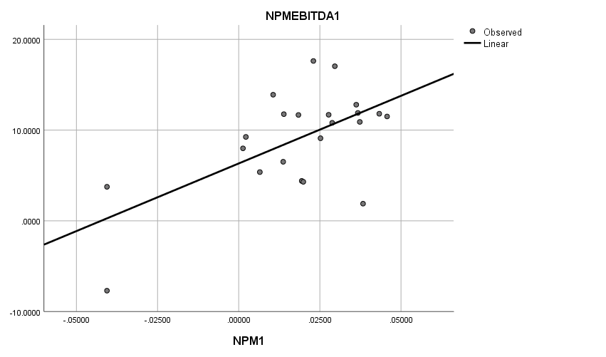
Figure 1: Plot of NPM1 vs. NPMEBITDA1 regression equation.

Table 7: Summary of NPM2 and NPMEBITDA2 regression models.

Table 8: Coefficients of NPM2 and NPMEBITDA2 regression models.

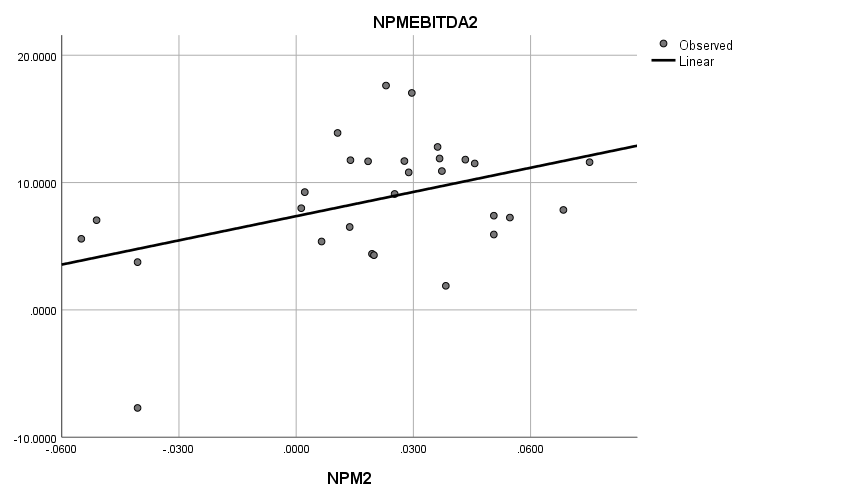
Figure 2: Plot of NPM2 vs. NPMEBITDA2 regression equation.

Table 9: Summary of GPM1 and GPMrevisedEBITDA1 regression models.

Table 10: ANOVA of GPM1 and GPMrevisedEBITDA1 regression models.

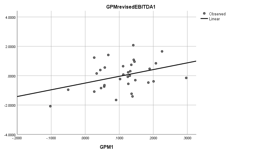
Figure 3: Plot of GPM1 vs. GPMrevisedEBITDA1 regression equation.

Table 11: Summary of GPM2 and GPMEBITDA2 regression models.

Table 12: Coefficients of GPM2 and GPMEBITDA2 regression models.

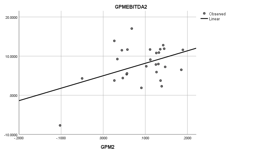
Figure 4: Plot of GPM2 vs. GPMEBITDA2 regression equation.

4. Discussion

Table 13: Table of parameters and their significance for each of the four sets of regression equations.

As the table 13 shown, this study concludes that both net profit margin and gross profit margin significantly affect EV/EBITDA, and both can reject the original hypothesis that the regression coefficient is zero. Moreover, net profit margin has more explanatory power on EV/EBITDA, and its correlation is more significant, indicating that net profit margin is a better financial factor to explain the firm's value than gross profit margin. Other things being equal, the greater the net profit margin and gross profit margin, the higher the enterprise value.

This study examines the relationship between two sets of regression analyses conducted on financial data. The findings indicate that as enterprises approach the range of net profit margin or gross profit margin where the majority of businesses are situated, the independent variable exhibits a stronger ability to explain variations in the dependent variable. Additionally, the significance of this relationship becomes more pronounced. This finding suggests that there is a stronger correlation between the observed pattern and the gross profit margin and net profit margin of general firms as they approach each other.

5. Conclusion

The U.S. construction industry faces a number of challenges, and this study begins by reviewing the various ways of studying the value of a firm. It points out their shortcomings, such as the need for more operationalization of qualitative models and the uncertainty of the value criterion. In order to address these limitations, the present study use regression analysis as a methodological approach to examine the financial aspects of the organization and formulate a regression equation. After the normal distribution test and heteroskedasticity test, one-way linear regression modeling is performed for EV/EBITDA, net profit margin, and gross profit margin, and two sets of data are selected within the same independent variable to make comparisons. In conclusion, it can be inferred that both the net profit margin and gross profit margin exert a favorable influence on EV/EBITDA, which serves as a metric for assessing the worth of a corporation. That net profit margin has a greater impact and is more significant. This pattern is more pronounced the closer to the range of gross and net profit margins where most firms are located.

This study still has some limitations. First, due to the restriction of the data sample, only March-April data were selected for this study. Follow-up should expand the sample size for a more comprehensive investigation. In addition, combining more factors for analysis is also a point where this study needs to go further.

The future research direction of this study lies in developing multiple linear regression equation modeling that integrates the effects of various financial factors on firm value. Structural equation modeling can also be established to measure the enterprise value with multiple elements and add different aspects to the model, such as the market size of the U.S. construction industry, the U.S. GDP, and other environmental factors. In this way, a more complete and comprehensive model can be established.

References

[1]. World Economic Forum & Boston Consulting Group (2016). Shaping the Future of Construction, A Breakthrough in Mindset and Technology.
[2]. Miles, S. J., & Van Clieaf, M. (2017). Strategic fit: Key to growing enterprise value through organizational capital. Business Horizons, 60(1), 55–65. https://doi.org/10.1016/j.bushor.2016.08.008
[3]. Jinfa, L., & Biting, L. (2017). Evaluation method of R&D investment value of intelligent manufacturing enterprise based on Growth Option. Procedia Engineering, 174, 301–307. https://doi.org/10.1016/j.proeng.2017.01.142
[4]. Diana, G. (2015). Repeated measures analysis on determinant factors of enterprise value. Procedia Economics and Finance, 32, 338–344. https://doi.org/10.1016/s2212-5671(15)01402-1
[5]. Vochozka, M., & Machová, V. (2017). Enterprise value generators in the building industry. SHS Web of Conferences, 39, 01029. https://doi.org/10.1051/shsconf/20173901029
[6]. Yoantika, A. F., & Susiswo. (2021). Comparing the principal regression analysis method with ridge regression analysis in overcoming multicollinearity on Human Development Index (HDI) data in Regency/City of east java in 2018. Journal of Physics: Conference Series, 1872(1), 012024. https://doi.org/10.1088/1742-6596/1872/1/012024
[7]. Luo,Xichang. (2020). Investment Merger and Acquisition Practice. Shanghai University of Finance and Economics Press.
[8]. Ma,Yongbin. (2020). Company Merger & Reorganization and Integration. Tsinghua University Press.
[9]. Bianconi, M., & Tan, C. M. (2017). Evaluating the instantaneous and medium-run impact of mergers and acquisitions on firm values. SSRN Electronic Journal. https://doi.org/10.2139/ssrn.2955524
[10]. Nariswari, T. N., & Nugraha, N. M. (2020). Profit growth : Impact of net profit margin, gross profit margin and total assests turnover. International Journal of Finance &, Banking Studies (2147-4486), 9(4), 87–96. https://doi.org/10.20525/ijfbs.v9i4.937
Cite this article
Chen,W. (2024). A Linear Regression-based Analysis of the Value of U.S. Construction Firms. Advances in Economics, Management and Political Sciences,72,23-33.
Data availability
The datasets used and/or analyzed during the current study will be available from the authors upon reasonable request.
Disclaimer/Publisher's Note
The statements, opinions and data contained in all publications are solely those of the individual author(s) and contributor(s) and not of EWA Publishing and/or the editor(s). EWA Publishing and/or the editor(s) disclaim responsibility for any injury to people or property resulting from any ideas, methods, instructions or products referred to in the content.
About volume
Volume title: Proceedings of the 2nd International Conference on Management Research and Economic Development
© 2024 by the author(s). Licensee EWA Publishing, Oxford, UK. This article is an open access article distributed under the terms and
conditions of the Creative Commons Attribution (CC BY) license. Authors who
publish this series agree to the following terms:
1. Authors retain copyright and grant the series right of first publication with the work simultaneously licensed under a Creative Commons
Attribution License that allows others to share the work with an acknowledgment of the work's authorship and initial publication in this
series.
2. Authors are able to enter into separate, additional contractual arrangements for the non-exclusive distribution of the series's published
version of the work (e.g., post it to an institutional repository or publish it in a book), with an acknowledgment of its initial
publication in this series.
3. Authors are permitted and encouraged to post their work online (e.g., in institutional repositories or on their website) prior to and
during the submission process, as it can lead to productive exchanges, as well as earlier and greater citation of published work (See
Open access policy for details).