1. Introduction

Happiness is a key aspect of human life. The United Nations celebrates the International Day of Happiness on March 20th each year to remind people of the importance of happiness [1]. Policymakers and scholars have tried hard to determine the essential factors affecting happiness, for proposing more effective public policy. Radcliff states that while many social factors such as education, wealth, and health are widely discussed, political factors did not enter the centre of literature discussion until the end of the 20th century [2]. In other words, people used to marginalize the importance of governance in promoting universal happiness. Headey and Wearing explain that the deemphasis of politics in affecting happiness is understandable because individuals are primarily concerned about personal variations in income, occupation, social relations, etc [3]. In contrast, they are more indifferent about the collective issues, such as the political issues affecting society. However, Radcliff argues that people will be happier when they are more satisfied with their social environment and political system, and political studies on happiness matter [2]. While there is increasing literature on relations between democracy and happiness, this essay focuses on another aspect of governance the quality of the government. This essay will take one of Paleologou’s approaches to measuring the quality of the government, which is the perception of corruption [4]. Finally, the research question of this paper is narrowed as follows: whether and how corruption affects happiness? This paper first reviews the development of literature on the study of happiness, corruption, and casual relations between them. Although the nature and direction of that impact are still being debated, the essay suggests an increasing consensus on the relevance of the two variables and gives a hypothesis by incorporating the analysis of literature and intuition. Next, the paper suggests the datasets, considering validity and reliability, and identifies controlling variables including GDP, democracy index and educational outputs. Finally, the paper raises a regression model and discusses the findings from the ordinary least square (OLS) test.

2. Literature Review

This part identifies the theoretical definition of happiness and corruption and reviews the development of academic literature not only on these factors themselves but also on possible relations between them.

2.1. Defining Happiness

Happiness can be measured by many metrics, encompassing multiple evaluations of one's life, including positive and negative aspects [5]. These evaluations might be either long-term or short-term. For instance, an individual can assess their subjective well-being based on the frequency of their happiness or negative emotions such as sorrow or fury in a short amount of time. Otherwise, subjective well-being can also be assessed by one’s long-time evaluation of their life.

Notice that this essay uses the term “life satisfaction” interchangeably with “happiness”, as Bok suggests the similarity of results when using two different words [6]. While some short-term research on subjective well-being tends to observe recent or current emotions of the participants, happiness serves as a long-term measure to reflect how people evaluate their overall lives regarding their personal goals or aspirations [5]. Therefore, this approach is more comprehensive and holistic.

2.2. Development of Happiness Study

The study on happiness boomed after the 1970s and the early studies intensively explored its relationship with economic factors [6]. Much research explains that economic development influences the standard of living, which is important in affecting happiness. The research suggests a strong positive correlation between the level of happiness and the national economy at a global level [7, 8]. Similarly, another famous study conveys the research at the domestic level, proving the positive correlation between personal income and hapiness in the U.S. (see Table 1 below) and most countries in the European Union [9].

Table 1: Levels of Satisfaction by Income Quartiles [10].

Nevertheless, Easterlin’s research contradicts the main strand of the study, proposing that there is no great difference in happiness between poor and rich countries [11]. He raises the “comparison theory” to explain that individual assessment of life is not the absolute value of income but contingent upon the “consumption norm”. Therefore, there should be an equal percentage of unhappy and happy people. Easterlin’s argument provides new insights into relations between material affluence and happiness, although his research is constantly challenged by other scholars, including Oswald who question the robustness and validity of his data [12].

The second strand of literature stresses on cultural approach or “cultural theory”. Inkeles highlights the importance of “culture” and “creeds” in affecting the national level of happiness [13]. Different from “comparison theory”, Inglehart acknowledges the potential for national variations in happiness, which results from collective and cognitive cultural norms [14]. However, both “comparison theory” and “cultural theory” reject that objective conditions have a substantial influence on variations in happiness. Both scenarios also neglect the role of politics. In the perspective of “comparison theory”, political outcome would just change the standard of consumption without affecting overall happiness; in “cultural theory”, political factors are ineffective in altering deeply ingrained cultural norms.

The third strand of literature gives more discussion on the relations between politics and happiness, which develops based on “liveability theory”. The theory supposes that physical that the more objective needs are satisfied, the happier people would be [15, 16]. In other words, life quality decides happiness. Veenhoven proves that individuals feel happier in communities that effectively meet the requirements of people [17]. The role of government is highlighted because happiness will vary based on the success of public policies in meeting populations’ needs. More recent research by Frey and Stutzer proves that the type of political system has an impact on their national level of happiness [18].

However, the literature on “liveability theory” has limitations. First, they mostly rely on rudimentary statistical methods, especially correlations. This paper will take one step further to do the OLS regression test beyond investigating correlations. Second, when considering economic advancement, the evidence that supports “liveability theory” becomes less persuasive [19, 20]. This echoes with Easterlin’s argument [11]. Therefore, this paper needs to consider economic performance as an important confounding variable.

2.3. Defining Corruption

Corruption is defined as misusing public authority for personal benefits, and it has various forms [21]. Firstly, corruption can exist in the process of policymaking, where the policymakers use their power to make political decisions favourable to certain interest groups. Second, corruption can also be observed in bureaucracy, where bureaucrats may use their authority for personal gain. Third, corruption can be found among legislators, whose voting decisions may be influenced by self-interest and sponsors. Corruption is influenced by various factors, including the advantages gained from corrupt practices, the value of economic privileges, the implementation of penalties and deterrents, the efficiency of political institutions, the presence of fair wages and lawful income, and societal norms [22].

There are two prevailing strands of literature on corruption. The first one focuses on the effects of corruption on the economic performance of developing countries. This includes its impact on bureaucratic efficiency, project selection, resource allocation, and more [23, 24]. The second body of work examines the welfare implications of corruption [25]. This paper will contribute to the latter strand of the literature, which is less discussed and needs more research.

2.4. Causal Relationship

The correlation between corruption and happiness is widely acknowledged. According to Ott, there is an independent association between technical quality and happiness in the political realm, regardless of cultural and national differences [26]. Nevertheless, the direction (positive/negative) of that influence is still unclear.

Some literature, particularly by liberal economists, hypothesised that corruption had a beneficial impact on happiness. Dreher & Gassebner contended that corruption diminishes the bureaucratic barriers and regulations associated with entrepreneurship, hence simplifying the process of establishing a business and enhancing its efficiency [27]. Paleologou’s analysis suggests that corruption can foster economic growth by prevailing over institutional inefficiencies through specific processes, thus enhancing people's happiness [4].

However, more scholars believe in the negative effects of corruption. First, citizens lose trust in government when they see corrupt officials [28]. Later research indicates that having confidence in others contributes to increased happiness [29]. Second, corruption reduces investment, which slows down the economy and has a detrimental effect on happiness [30]. Third, corruption worsens the income inequality [31]. The following research proves that economic inequality directly decreases happiness [32]. Finally, corruption distorts the allocation of government funds by reducing allocations to the education sector and increasing allocations to the military sector [33, 34].

2.5. Hypothesis

This paper corresponds with the second strand of the literature in the above section, hypothesizing that the lower the level of corruption, the higher the level of happiness, and vice versa. Notably, the paper needs to control many other variables, as other literature argues for the influence of other factors on happiness.

3. Methodology

This study will use aggregate national indicator of 133 countries in the world, trying to give a holistic view of the happiness-corruption relationship internationally. This study would have attempted to find data that covers most of the countries in the world. However, due to conflict, poverty, and turbulence, etc., data of many countries, mostly undeveloped nations, are missing.

3.1. OLS Test in Stata and Theorised Model

Stata will be used to managing and analysing the large datasets, as it is known for its statistical accuracy and reliability. Ordinary least squares (OLS) test will be used in this paper, with a proposed model below.

\( Hapiness=a+b\times Corruption+\mu \) (1)

Where: \( a \) is constant, \( b \) is regression coefficient, \( \mu \) is unsystematic error.

3.2. Dataset

The dataset and resource of dependent variables, independent variables, and other controlling variables will be discussed below.

3.2.1. Dependent Variables

National indicator is comprehensive and integrated to inform policymaking [35]. Therefore, the paper uses the Happiness Index (HPI) from the World Happiness Report 2023. The report is produced by the United Nations Sustainable Development Solutions Network and uses data from the Gallup World Poll. It looks at the average “life evaluation” score for each country. Around 1,000 participants in every nation were surveyed to assess their overall life using a scale of 0 to 10.

The World Happiness Report has high face validity, as it measures self-reported happiness, which aligns with the definition of happiness raised by Diener [5]. Conducting cross-national and macro-level analysis might circumvent the issues of sampling bias that can happen in micro-level analysis which only selects a small sample. Although some scholars prefer deconstructing aggregate indicators of happiness and applying multilevel analysis of the local, regional, and communal aspects, the process is laborious and time-consuming [19].

The resource is reliable that researcher of the report comes from the SDSN. It is a global initiative created by the United Nations, so the paper assumes the data are credible and reliable. Also, the primary data source, the Gallup World Poll, uses a consistent survey methodology across countries, which helps ensure reliability.

3.2.2. Independent variables

It is difficult to create scientific and objective measurements of corruption since, in most cases, it entails unlawful and intentionally hidden behaviours that are only revealed through scandals or legal action. This paper will utilise the data from the Corruption Perceptions Index 2023 (CPI) compiled by Transparency International, an organisation that is also a member of the SDSN. The metric assesses the extent to which professionals and businesspeople perceive corruption within the public sector of each country. Perceived corruption increases as the score decreases. The Corruption Perceptions Index (CPI) is a measure developed by Transparency International to assess levels of corruption.

The resource has high validity. Each country’s score is derived by aggregating data from at least three data sources obtained from 13 distinct corruption surveys and evaluations. This approach provides a more comprehensive understanding of the situation compared to relying on a single index. Some people criticized CPI for not measuring actual corruption directly, which harms its content validity since perceptions might not align with reality. However, perceptions are crucial because they can influence investment, governance, and public trust, which are integral to the impact of corruption.

The resource is reliable that Transparency International uses a consistent methodology for compiling the index each year. Data from several reliable organisations, such as the World Bank and the World Economic Forum, are compiled to create these data sources.

3.3. Controlling Variables

The paper will control 3 additional variables beyond the given independent variables, hopefully mitigating the omitted-variable bias. While there may be additional factors that influence happiness, these are the most crucial and concerning ones.

The democracy index, another facet of governance, has been extensively associated with happiness, because it represents the freedom of political participation and the involvement in decision-making processes [19]. Hence, this paper will include the Freedom House Index (FHI) in the model. Freedom House index is an integrated measurement of political rights and civil liberties, which are important sub-factors of democracy.

Otherwise, as the literature debating on “comparison theory”, economic factors will be considered as an essential confounding variable. Hence, we incorporate GDP per capita (referred to as GDP below) provided by the World Bank into our model. The World Bank uses standardized definitions and methodologies that align with international conventions, such as those provided by the United Nations, which ensures the data accurately reflects economic activity. The data is designed to be comparable across countries, making it a valuable tool for cross-national studies.

Following Mauro’s point that corruption leads to decreasing happiness, this paper controls education in the model. This paper follows Chakravarthi’s method of calculating the education index (EDI): first collects cross-national statistics of “expected years of schooling” and “mean years of schooling” from United Nations Development Programmes (UNDP), and then uses the formulation “( \( \frac{EYS}{18}+\frac{Mys}{15})/2 \) ” to get the EDI [36]. The Index is valid for comparing educational attainment across countries, particularly when considering the quantity of education (years of schooling). Its reliability is supported by consistent collection methods, regular updates, and transparency in its methodology.

Therefore, the final version of the theorised model will be:

\( HPI=a+b1\times CPI+b2\times FHI+b3\times EDI+b4\times GDP+\mu \) (2)

Where: \( a \) is constant, \( b \) is regression coefficient; \( \mu \) is unsystematic error

4. Findings and Analysis

This part starts by solely considering relationship between CPI and HPI, and then controlling variables will be added into the model one by one to see the change of the key statistics.

4.1. Bivariate Relationship between CPI and HPI

Before doing the regression test, the research first runs a correlation test (see Table 2).

Table 2: correlation coefficient

Then a scatterplot is drawn between CPI and HPI (see Figure 1) to have a preview of the data.

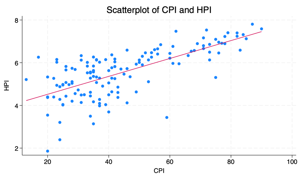
Figure 1: HPI vs CPI Scatterplot with a line of best fit.

The results show a strong positive relationship between HPI and CPI (r=0.6861). Then, the OLS regression starts by only testing CPI in the model (see Table 3).

Table 3: Regression test result between CPI and HPI

4.1.1. Interpretation

CPI is a significant predictor of HPI. First, the p-value for the CPI coefficient is 0.000, meaning that it is statistically significant at any conventional level (e.g., 1%, 5%, 10%). This suggests that the result of relationship between CPI and HPI is unlikely detected by chance. Besides, the p-value associated with the F-statistic is 0.0000 indicating that the model is statistically significant at the 1% level. Finally, a t-value of 11.23 is very large.

The result reapproves the strong positive relationship between CPI and HPI, and the explanatory power of CPI on HPI is quite high. First, for every one-unit increase in CPI, the HPI is expected to positively increase by about 0.042 units, holding all else constant. Second, a beta of 0.6976439 suggests that for one standard deviation increase in CPI, the HPI is expected to increase by approximately 0.698 standard deviations, holding other factors constant. Third, approximately 48.67% of the variance in HPI can be explained by CPI.

4.2. Adding Controls

The OLS test continues by adding other controlling variables into the model to see their effect on the relationship between HPI and CPI. The focus will be on standardized beta value, as it allows for comparison between the effects of different predictors.

4.2.1. Adding FHI

FHI is added into the model first (see Table 4).

Table 4: The result of controlling FHI.

CPI remains a significant predictor of HPI. The positive coefficient and high beta value indicate that CPI still has a strong positive relationship with HPI, meaning that as CPI increases, HPI also tends to increase. FHI is not statistically significant at the 5% level (p-value > 0.05) but is close to being significant at the 10% level. The positive coefficient and beta suggest that there is a potential positive relationship between FHI and HPI, although this relationship is weaker compared to CPI.

Regarding the whole model, approximately 49.90% of the variance in HPI is explained by the model, which includes both CPI and FHI. This is a slight improvement from the previous model that only included CPI. Otherwise, the overall F-test is significant (Prob > F = 0.0000), indicating that the model is statistically significant in explaining the variance in HPI.

4.2.2. Adding EDI

EDI is then added into the model (see Table 5).

Table 5: The result of controlling EDI.

First, CPI remains a significant predictor of HPI. However, its influence has decreased compared to previous models (as indicated by the lower coefficient and beta). The positive relationship still holds, meaning that as CPI increases, HPI tends to increase. Second, FHI is not statistically significant (p-value > 0.05), indicating that it does not have a strong or significant impact on HPI in this model. Its beta value is also relatively low, suggesting a weaker relationship with HPI. Third, EDI is a significant predictor of HPI with the highest beta value, suggesting that this new variable is an important factor in predicting HPI. The low p-value suggests the result is statistically significant and unlikely detected by chance.

Regarding the whole model, approximately 63.03% of the variance in HPI is explained by the model, which includes CPI, HPI, and EDI. This represents a significant improvement in model fit compared to previous models, proving the importance of education in predicting happiness. Otherwise, the overall F-test is significant (Prob > F = 0.0000), confirming that the model is statistically significant in explaining the variance in HPI.

4.2.3. GDP

Finally, GDP is added into the model (see Table 6).

Table 6: The result of controlling EDI.

First, CPI is no longer a significant predictor of HPI after adding GDP to the model. The p-value is very high, indicating that the weak relationship between CPI and HPI is likely detected by chance. CPI has almost no explanatory power in this context. The beta value is also very low, suggesting a negligible relationship with HPI. Second, FHI is marginally significant, with a p-value close to 0.05. The beta value indicates a relatively weak relationship with HPI, but it still has some relevance in the model. Third, EDI remains a highly significant predictor of HPI. The large coefficient and beta value indicate a strong positive relationship, like previous models. Finally, GDP is a significant predictor of HPI. The positive coefficient suggests that as GDP increases, HPI also tends to increase. It has the highest beta value in the model, indicating its importance and strong explanatory power in predicting happiness. It can be assumed that a large part of the explanatory power of CPI in the previous model is associated with the variations in GDP. This may cause the problem of multicollinearity, which will be diagnosed in the paper later.

Regarding the whole model, approximately 66.00% of the variance in HPI is explained by the model, which now includes CPI, FHI, EDI, and GDP. This shows a further improvement in model fit compared to previous models. Otherwise, the overall F-test is significant (Prob > F = 0.0000), confirming that the model is statistically significant in explaining the variance in HPI.

4.3. Postdiagnosis

In this section, the paper will do postdiagnosis to identify the potential issue of the chosen variables and model. Multicollinearity, mean independence, and homoscedasticity will be discussed.

4.3.1. Multicollinearity of Variables

The variance inflation factor (VIF) test is run to test if the variables are highly correlated (see Table 7).

Table 7: VIF Test on CPI, GDP, EDI, and FHI.

While the VIF for CPI is slightly above 5, it doesn’t reach a level that typically requires corrective action (e.g., removing variables, combining variables, or using techniques like ridge regression). The other variables are in acceptable ranges that are smaller than 5. The model appears to be stable, with no severe multicollinearity that would undermine the reliability of the coefficient estimates. However, the high VIFs of CPI and GDP show that they are highly correlated, which explains the statistical insignificance of CPI and the substantial fall of beta when GDP is included in the model.

4.3.2. Mean Independence and Homoscedasticity

The residuals-versus-predictor plot and residuals-versus-fitted values plot are made (see Figure 2 and 3).

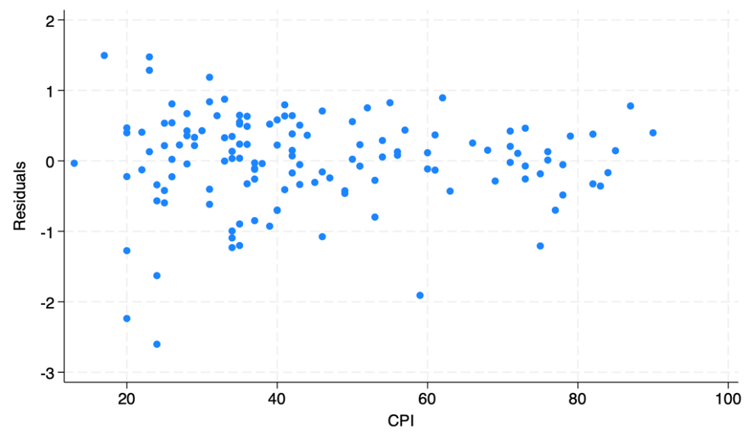
Figure 2: Residuals vs. CPI.

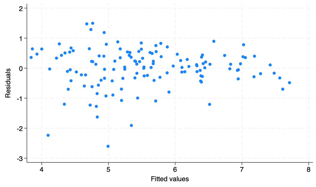
Figure 3: Residual vs. fitted values.

Mean independence is crucial when considering whether an explanatory variable in a regression model can be treated as exogenous. In both graphs, the residuals show little change when CPI moves, apart from a few outliers in the lower left corner. Therefore, the CPI is independent of the error term, which suggests that the variable is exogenous and does not suffer from endogeneity.

To meet the assumption of homoscedasticity, the residuals should be normally distributed and have the same variance at each level of the CPI. Both graphs show that the model is well-fitted. Thus, the assumption of homoscedasticity is satisfied.

5. Conclusion

This paper does a cross-national study on how corruption impacts happiness. Scholars generally agree that corruption affects happiness, as shown in the research review. However, the direction of causal relations is debatable. To solve this puzzle, this essay conducts an OLS test on the two variables and controls other relevant variables. The hypothesis of this paper that corruption has negative result on happiness is supported at the first stage by the test result, which persists after controlling the democracy and education index. However, CPI becomes statistically insignificant after taking GDP into account. The test result can be explained as follows. First, it can be the result of measurement error in methodology. Nevertheless, we are sceptical of this explanation because the p-value is so high (0.928). Second, there can be a spurious relationship between happiness and corruption. However, the literature review by scholars have widely acknowledged the causal relationship between the two variables. The last explanation is more convincing in this context: GDP serves as an intervening variable between happiness and corruption. It corresponds with the high correlation the VIF test results show. Otherwise, a large amount of study on corruption centers around economy, such as its effect on decreasing investment and income inequality. This paper may have limitations. First, due to the time and space limit, this paper cannot delve into the intricate relationship between variables, particularly GDP and CPI. Second, the dataset of this study focuses on a relatively short time performance of 2022-2023. However, the analysis of this paper serves as an initial exploration into these dynamics, offering foundational insights that can be expanded upon in future research. For instance, the problem of multicollinearity can be mitigated by recoding and combining variables GDP and CPI. To get a more holistic view of the issue, later research can use datasets with longer time spans based on the methodology of this paper. Researchers and policymakers can build on these findings to further understand the factors driving happiness, ultimately contributing to more informed decision-making on anti-corruption campaigns and promoting happiness.

References

[1]. Helliwell, J., Layard, R., & Sachs, J. (2012). World happiness report 2012. New York: Sustainable Development Solutions Network.
[2]. Radcliff, B. & Shufeldt, G. (2016). Direct Democracy and Subjective Well-Being: The Initiative and Life Satisfaction in the American States. Social Indicator Research 128, 1405–1423. https://doi.org/10.1007/s11205-015-1085-4
[3]. Headey, B., & Wearing, A. (1992). Understanding happiness: A theory of subjective well-being. Melbourne, Australia: Longman Cheshire Pty Limited.
[4]. Paleologou, S.M. (2022). Happiness, democracy and socio-economic conditions: Evidence from a difference GMM estimator. Journal of Behavioral and Experimental Economics, 101.
[5]. Diener, E., Oishi, S., & Lucas, R. (2011). Subjective well-being: The science of happiness and life satisfaction. In S. J. Lopez, & C. R. Snyder (Eds.), The Oxford handbook of positive psychology (pp. 187–194). Oxford: Oxford University Press.
[6]. Bok, D. (2010). The politics of happiness : What government can learn from the new research on well-being. Princeton University Press.
[7]. Blanchflower, D.G. and Oswald, A.J., (2004). Well-being over time in Britain and the USA. Journal of public economics, 88(7-8), pp.1359-1386.
[8]. Veenhoven, R. and Ehrhardt, J., (1995). The cross-national pattern of happiness: Test of predictions implied in three theories of happiness. Social indicators research, 34, pp.33-68.
[9]. Tella, R.D. and MacCulloch, R., (2006). Some uses of happiness data in economics. Journal of economic perspectives, 20(1), pp.25-46.
[10]. Easterlin, R. (1974). Does economic growth improve the human lot? Some empirical evidence. In P. A. David & M. W. Reder (Eds.), Nations and households in economic growth: Essays in honour of Moses Abramovitz. New York: Academic Press.
[11]. Tella, R.D., MacCulloch, R.J. and Oswald, A.J., 2003. The macroeconomics of happiness. Review of Economics and Statistics, 85(4), pp.809-827.
[12]. Oswald, A.J., (1997). Happiness and economic performance. The economic journal, 107(445), pp.1815-1831.
[13]. Inkeles, A. (1997). National Character. New Brunswick, NJ: Transaction.
[14]. Inglehart, R., (2018). Culture shift in advanced industrial society. Princeton University Press.
[15]. Veenhoven, R., (1994). Is happiness a trait? Tests of the theory that a better society does not make people any happier. Social indicators research, 32(2), pp.101-160.
[16]. Schyns, P., (1998). Crossnational differences in happiness: Economic and cultural factors explored. Social Indicators Research, 43, pp.3-26.
[17]. Veenhoven, R., (1995). World database of happiness. Social Indicators Research, 34, pp.299-313.
[18]. Frey, B., & Stutzer, A. (2009). Should national happiness be maximized? In D. Amitava, & B. Radcliff (Eds.), Happiness, economics and politics. Cheltenham, U.K. and Northampton, MA: Edward Elgar.
[19]. Veenhoven, R., (1997). Advances in understanding happiness. Revue québécoise de psychologie, 18(2), pp.29-74.
[20]. Radcliff, B. (2001), "Politics, markets, and life satisfaction: The political economy of human happiness", The American Political Science Review, vol. 95, no. 4, pp. 939-952.
[21]. Lambsdorff, J.G., (2003). How corruption affects productivity. Kyklos, 56(4), 457-474.
[22]. Arvin, M. & Lew, B. (2014) "Does income matter in the happiness-corruption relationship?", Journal of Economic Studies, vol. 41, no. 3, pp. 469-490.
[23]. Rose-Ackerman, S. (1997) Corruption: Causes, consequences and cures: Paper presented at the Institute for Contemporary Studies and National Strategy Information Center Conference, ‘Challenge of Corruption,’ Mexico, March 1997. Trends in organized crime. [Online] 3 (1), 109–111.
[24]. Mauro, P. and Driscoll, D.D., (1997). Why worry about corruption? (Vol. 6, pp. 1-19). Washington, DC: International Monetary Fund.
[25]. Gupta, S. (1998) The IMF and the poor / Fiscal Affairs Department. International Monetary Fund.
[26]. Ott, J.C. (2010) Good Governance and Happiness in Nations: Technical Quality Precedes Democracy and Quality Beats Size. J Happiness Stud, 11, 353–368. https://doi.org/10.1007/s10902-009-9144-7.
[27]. Dreher, A., & Gassebner, M. (2013). Greasing the wheels? The impact of regulations and corruption on firm entry. Public Choice, 155, 413–432.
[28]. Tay, L., Herian, M. N., & Diener, E. (2014). Detrimental effects of corruption and subjective well-being: Whether, how and when. Social Psychological and Personality Science, 5(7), 751–759.
[29]. Hommerich, C., & Tiefenbach, T. (2018). Analyzing the relationship between social capital and subjective well-being: The mediating role of social affiliation. Journal of Happiness Studies, 19(4), 1091–1114.
[30]. Sacks, D. W., Stevenson, B., & Wolfers, J. (2010). Subjective well-being, income, economic development and growth. NBER Working Papers Series.
[31]. Glaeser, E. L., & Saks, R. E. (2006). Corruption in America. Journal of Public Economics, 90(6–7), 1053–1072.
[32]. Schröder, M. (2018). Income inequality and life satisfaction: Unrelated between countries, associated within countries over time. Journal of Happiness Studies, 19(4), 1021–1043.
[33]. Mauro, P. (1998). Corruption and the composition of government expenditure. Journal of Public Economics, 69(2), 263–279.
[34]. Gupta, S., de Mello, L., & Sharan, R. (2001). Corruption and military spending. European Journal of Political Economy, 17(4), 749–777.
[35]. Kesebir, P., & Diener, E. (2008). In pursuit of happiness: Empirical answers to philosophical questions. Perspectives on Psychological Science, 3(2), 117–125.
[36]. Jin, H., Qian, X., Chin, T., & Zhang, H. (2020). A global assessment of sustainable development based on modification of the human development index via the entropy method. Sustainability, 12(8), 3251.
Cite this article
Fang,C. (2024). A Cross-national Study on How Corruption Affects Happiness. Lecture Notes in Education Psychology and Public Media,64,80-92.
Data availability
The datasets used and/or analyzed during the current study will be available from the authors upon reasonable request.
Disclaimer/Publisher's Note
The statements, opinions and data contained in all publications are solely those of the individual author(s) and contributor(s) and not of EWA Publishing and/or the editor(s). EWA Publishing and/or the editor(s) disclaim responsibility for any injury to people or property resulting from any ideas, methods, instructions or products referred to in the content.
About volume
Volume title: Proceedings of the 2nd International Conference on Global Politics and Socio-Humanities
© 2024 by the author(s). Licensee EWA Publishing, Oxford, UK. This article is an open access article distributed under the terms and
conditions of the Creative Commons Attribution (CC BY) license. Authors who
publish this series agree to the following terms:
1. Authors retain copyright and grant the series right of first publication with the work simultaneously licensed under a Creative Commons
Attribution License that allows others to share the work with an acknowledgment of the work's authorship and initial publication in this
series.
2. Authors are able to enter into separate, additional contractual arrangements for the non-exclusive distribution of the series's published
version of the work (e.g., post it to an institutional repository or publish it in a book), with an acknowledgment of its initial
publication in this series.
3. Authors are permitted and encouraged to post their work online (e.g., in institutional repositories or on their website) prior to and
during the submission process, as it can lead to productive exchanges, as well as earlier and greater citation of published work (See
Open access policy for details).