1. Introduction

China’s soaring housing prices in recent decades have significantly influenced the socioeconomic landscape, making it increasingly difficult for young adults to purchase homes and form families. As housing affordability declines, many are delaying or opting out of marriage. While previous research has explored factors such as economic stability and social attitudes affecting marriage rates, fewer studies have examined the long-term impact of rising housing costs within China’s unique socioeconomic context, highlighting a critical research gap.This study investigates the effect of housing prices on marriage rates in China using provincial panel data from 2005 to 2022. By employing regression models and incorporating control variables such as per capita GDP, divorce rates, and birth rates, the study seeks to provide robust insights into the dynamic relationship between housing costs and marriage decisions.

The research offers valuable insights for policymakers, emphasizing the need to address the societal impact of rising housing prices. By understanding their influence on marriage trends, targeted policies in real estate and social welfare can be developed to reduce financial pressures, support family formation, and promote long-term social and economic stability.

2. Literature Review

Existing literature extensively explores the relationship between housing prices and marriage rates but reveals notable gaps. Many studies, such as those based on Becker’s family economics theory , focus on theoretical frameworks without sufficient empirical support[1]. Research by Hong Caini and Zheng Yiping examines housing price impacts on marriage using older or region-specific data, limiting broader applicability[2][3]. Additionally, most studies emphasize short-term price fluctuations, neglecting the long-term effects of rising housing prices on trends in marriage and family planning. While Yi Junjian and Liu Xiaoting have linked housing prices to fertility rates, empirical evidence on their influence on marriage decisions remains limited[4][5].

Recent work by Lin Juan and Wei Jiamin uses provincial panel data to investigate the relationship between housing prices and first marriage rates from 2010 to 2016. While their study provides valuable insights and robust statistical significance for factors like birth rate and per capita GDP, it is limited by its timeframe and neglects critical variables, such as the proportion of the marriageable population and the gender ratio[6].

Building on this foundation, the present study incorporates a panel data regression model with individual and time-fixed effects to control for unobserved heterogeneity. Additionally, it establishes a nonlinear relationship between housing price fluctuations and marriage rates through a polynomial regression model, providing a more precise and comprehensive understanding[7]. These contributions enhance theoretical and empirical perspectives, offering actionable insights for housing and population policy development[8].

3. Data and Methodology

3.1. Variable Selection

This study have selected multiple economic and social variables to explore their impact on marriage rates. Specifically, marriage rate is chosen as the dependent variable, while average housing sales price is selected as the primary explanatory variable. Additionally, birth rate, divorce rate, per capita GDP, CPI, average education level of individuals aged 6 and above, population proportion of young and middle-aged adults (aged 20-49), and the absolute deviation of the sex ratio from the normal value of 105 are chosen as control variables. The following table1 provides statistics for each of these variables:

Table 1: Introduction of different variable codes

Note: In the predicted direction of change, "+" indicates that as the variable increases, the marriage rate also increases;

"-" indicates that as the variable increases, the marriage rate decreases.

3.2. Data Sources

The data used in this study are sourced from the "China Statistical Yearbook," the "China Population Census Yearbook," as well as bulletins and statistical data released by the National Bureau of Statistics and the Ministry of Civil Affairs. These data cover nationwide information on housing prices, marriage rates, divorce rates, birth rates, and other economic and social indicators from 2005 to 2022. The "China Statistical Yearbook" and the "China Population Census Yearbook" provide our research with official and meticulously calculated population and economic data, ensuring the authority and accuracy of the data. Bulletins from the National Bureau of Statistics and the Ministry of Civil Affairs further provide the latest statistical data on various socioeconomic activities, including residents' income, consumption levels, price indices, and educational status, providing a solid data foundation for analyzing the relationship between housing prices and marriage rates[9].

\( Marriage Rate=\frac{Newly Married×2}{Populatio{n_{Last year}}+Populatio{n_{This year}}}×100\% \) (1)

Since the marriage rate (dependent variable) and the average education level of individuals aged 6 and above (control variable) cannot be directly obtained from raw data, this study can indirectly calculate them using the following formulas, based on the number of marriage registrations, the population at the beginning and end of the year, and the number of individuals who have never attended school, only attended primary school, attended junior high school, attended high school, as well as those with college, undergraduate, and graduate degrees.

\( Average Years of Education=\frac{+ \begin{array}{c} Primary Population×6+Middle Population×9 \\ (High Population+Vocational Population)×12 \\ +College Population×16 \end{array} }{Total Population } \) (2)

The calculation of the marriage rate standardizes the number of first marriages each year to the total population in the same age group. Specifically, it is calculated by multiplying the number of first marriages within the year by 2 (since a marriage involves two individuals) and then dividing by the total unmarried and married population within the same age bracket. Regarding the age ranges considered for different time periods, data from 2005 to 2014 include populations aged 6-9 and 12-16, while data from 2015 to 2022 cover populations aged 6-9 and 12-19. This distinction arises due to potential changes in the scope and standards of statistical data collection over time.

4. Empirical Result

4.1. Descriptive statistics

4.1.1. Correlation Analysis

There is a clear negative correlation between housing prices and marriage rates, suggesting that rising housing prices may suppress marriage rates, supporting the idea that higher housing costs increase marriage expenses for young people. The divorce rate also shows a negative correlation with marriage rates, indicating that marriage instability may reduce confidence in marriage.

Birth rates and marriage rates display a positive correlation, implying that regions with higher birth rates tend to have higher marriage rates. The consumer price index (CPI) appears negatively correlated with marriage rates, suggesting that rising living costs may delay marriage. Higher education levels also show a negative correlation with marriage rates, indicating that more education may delay marriage decisions. Additionally, the proportion of young adults is positively correlated with marriage rates, while gender imbalance negatively correlates with marriage rates.

These findings align with theoretical expectations and support further quantitative analysis.

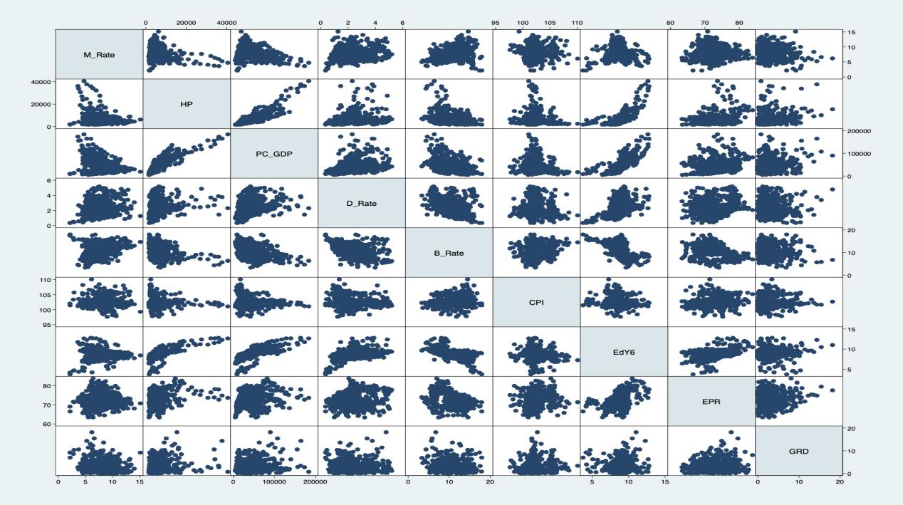
Figure 1: Matrix scatter plot of variable correlation

4.1.2. Descriptive Statistics

The average marriage rate is 7.995 with a standard deviation of 2.044, indicating regional differences. The skewness is 0.236,

and kurtosis is 3.104, suggesting a slightly right-skewed but nearly normal distribution.

The average housing price is 6542.793 yuan, with a high standard deviation of 5301.94 and a maximum of 40526 yuan, indicating large price fluctuations. The skewness of 3.154 and kurtosis of 16.063 show an extremely right-skewed distribution.

The average divorce rate is 2.403, with a balanced distribution. Birth rates average 10.934, with near-symmetry in distribution (skewness -0.19). CPI has a slight right skew (0.793), and education years average 8.775, showing a left-skewed distribution.

The proportion of marriageable population averages 72.744, while the gender ratio deviation shows serious imbalances in some regions. The per capita GDP averages 45957.24 yuan, with a highly right-skewed distribution.

Table 2: Descriptive statistics of each variable

4.2. Heteroscedasticity Test

In order to initially assess whether the heteroskedastic robust form of standard deviation is needed in the subsequent regression model, we conducted a heteroskedasticity test in the regression of marriage rates on housing prices, and the results are as follows(see table 3):

White's test for Ho: homoskedasticity

against Ha: unrestricted heteroskedasticity

chi2(2) = 13.13

Prob > chi2 = 0.0014

Table 3: Cameron & Trivedi's decomposition of IM-test

According to White's test, the test statistic follows a chi-squared distribution with 2 degrees of freedom (12.63), and the corresponding p-value is 0.0014, which is much smaller than the commonly used significance level of 0.05. This result rejects the null hypothesis of constant residual variance, indicating the presence of heteroscedasticity in the model, meaning that the residual variance changes with the explanatory variables.

4.3. Regression Analysis

4.3.1. Linear model

First, a linear model was used to analyze the impact of housing prices on marriage rates. In Model 1, the results showed that for every unit increase in housing prices, the marriage rate significantly decreased (coefficient = -0.000***), but the model's goodness of fit was low (7.7%), indicating the presence of omitted variables. After adding per capita GDP in Model 2, although per capita GDP also had a negative impact on marriage rates, the effect of housing prices remained significant. Model 3 introduced divorce rates, indicating a significant positive correlation between increasing divorce rates and marriage rates, possibly because remarriage offsets the negative effects of housing prices.

Table 4: Regression analysis results of linear model

Robust standard errors in parentheses

*** p<0.001, ** p<0.01, * p<0.05

After including birth rates in Model 4, the model's explanatory power increased to 23.7%, with birth rates positively correlated with marriage rates. Models 5 and 6 added CPI and education level, with education level significantly increasing marriage rates (coefficient = 0.900***), and the model's goodness of fit reached 33.8%. Models 7 and 8 introduced the proportion of eligible populations and the deviation in gender ratio, with the proportion of eligible populations significantly enhancing marriage rates.

Ultimately, the explanatory power of Model 8 was superior to that of other models (R-squared = 36.2%), but the coefficients for CPI and the deviation in gender ratio were not significant. Therefore, by comparing Models 7, 8, and subsequent models that eliminated non-significant variables, Model 10 was determined to be the optimal linear regression model(see table5).

Table 5: Comparison of three Models regression results

Robust standard errors in parentheses

*** p<0.001, ** p<0.01, * p<0.05

4.3.2. Nonlinear Model

In the analysis of nonlinear models, taking the logarithm of housing prices addresses the issue of underestimated coefficient estimates in the original model. The linear-logarithmic model effectively optimized this problem in the 11th regression. Models 12 and 13 are the logarithmic-linear model and the double-logarithmic model, respectively, both significant, but for the sake of simplifying the analysis, the linear-logarithmic model was selected. Model 14 introduces a polynomial of the logarithm of housing prices (squared and cubic terms), with coefficients for the first, second, and third terms being 241.057***, -26.282***, and 0.948***, significantly enhancing the model's goodness of fit to 47.4% (compared to 38.7% for model 13). Models 15-19 add interaction terms to the linear-logarithmic model.

Model 15's "ln housing price_per capita GDP" explores the interactive effects of housing prices and economic levels; model 16's "ln housing price_divorce rate" analyzes the suppressive effect of high housing prices on marriage rates in the context of high divorce rates; model 17's "ln housing price_birth rate" reflects that high birth rate areas may encourage family formation even at high housing prices;

Model 18's "ln housing price_years of education for those over six" investigates the mitigating effect of education levels on housing prices[10]; and model 19's "ln housing price_ratio of marriageable population" shows that under high ratios of marriageable population, high housing prices suppress marriage rates[11]. The regression results for interaction terms indicate that the interaction terms "ln housing price_divorce rate" (-0.585***) and "ln housing price_years of education for those over six" (-0.736***) in models 16 and 18 are significant at the 1% level, while other interaction terms are not significant. The 20th regression integrates these two significant interaction terms, and the joint hypothesis test (F = 28.12) is significant, indicating that both are non-zero; therefore, model 20 is selected as the optimal nonlinear regression model.

Table 6: Regression analysis results of nonlinear model

Robust standard errors in parentheses

*** p<0.001, ** p<0.01, * p<0.05

4.4. Multicollinearity Test

Table 7: Test results of Multicollinearity of Model 10

This paper conducted a multicollinearity test on the optimal model 10 in the linear regression analysis. The VIF values for all variables in the model are below 10, with an average VIF of 2.92, indicating that there is no severe multicollinearity problem. The collinearity effect among explanatory variables is relatively minor.

4.5. Panel Regression

4.5.1. Hausman test

It was conducted to compare fixed and random effects models, yielding a chi-squared value of 80.98 with a p-value < 0.0001, indicating that the fixed effects model is more suitable for this data. The fixed effects estimates for key variables such ln(HP), PC_GDP , D_Rate, and marriage rate differ significantly from random effects estimates, suggesting correlation between explanatory variables and unobserved individual effects. Thus, the fixed effects model effectively controls for unobserved heterogeneity, providing more consistent estimates.

Table 8: Results of the Housman test

chi2(5) = (b-B)'[(V_b-V_B)^(-1)](b-B)= 80.98 ; Prob>chi2 = 0.0000

4.5.2. Fixed Effects Analysis

In terms of coefficient significance, variables in Models 21 and 22 have statistically significant estimates, allowing the null hypothesis of zero coefficients to be rejected with confidence. Model 21 exhibits a higher goodness-of-fit (71.7%) compared to Model 22 (61.8%), indicating that Model 21 provides better estimates when only accounting for unobserved variables that vary by individual and not by time. Therefore, Model 21, which incorporates individual fixed effects, is considered the superior model for this analysis.

In comparison to Models 21 and 22, which include individual fixed effects, Model 23 introduces a dummy variable for each year from 2006 to 2021 to account for unobserved variables that vary over time but not by individual. This approach adds an excessive number of explanatory variables, which reduces degrees of freedom, increases the variance of estimates, and decreases model efficiency. Furthermore, with the inclusion of time-fixed effects in Model 23, the coefficients for divorce rate and the interaction term (lnHP_D_Rate) lose significance, and the newly introduced dummy variables for 2007, 2015, and 2016 fail to reject the null hypothesis of zero coefficients. Therefore, this study conclude that Model 23 performs worse than Models 21 and 22, suggesting that the analysis of housing prices impact on marriage rates should focus more on unobserved variables that vary by individual but not over time

In Model 24, this study include two sets of dummy variables to represent both individual fixed effects and time fixed effects. In Model 25, this study apply time averaging and construct a mean-deviation equation to achieve individual demeaning, eliminating unobserved variable bias that varies by individual but not over time. Additionally, this study introduce T-1 dummy variables to remove unobserved biases that vary over time but not by individual, thereby avoiding perfect multicollinearity. However, regardless of the calculation method used, adding both individual and time fixed effects causes the coefficients of control variables, such as the eligible population ratio and the interaction term(lnHP_D_Rate), to lose significance. Based on this analysis, this study ultimately select Model 21 as the optimal model for the panel data regression analysis.

Table 9: Comparative analysis of Panel Data Regression

Robust standard errors in parentheses

*** p<0.001, ** p<0.01, * p<0.05

5. Conclusion and Policy Implications

The findings of this study reveal that housing prices exert a significant suppressive effect on marriage rates, with the relationship quantified by the polynomial regression model:

\( \hat{M\_Rate}=226.857(ln{HP})-25.270{(ln{HP})^{2}}+0.971{(ln{HP})^{3}}-0.0001(PC\_GDP)+4.284(D\_Rate)+0.245(B\_Rate)+7.080(EdY6)+0.300(EPR)-0.452((lnHP)*(D\_Rate))-0.789((ln{HP})*(EdY6)) \)

This formula encapsulates the nonlinear dynamics between housing prices and marriage rates, highlighting the diminishing returns of increased housing costs on family formation. Despite its robustness, this study has certain limitations. Firstly, while provincial panel data captures macroeconomic trends, it may overlook micro-level variations such as urban-rural disparities or cultural influences on marriage. Secondly, the study’s reliance on secondary data sources could limit the depth of insights into behavioral and psychological factors driving marriage decisions. Future research could address these gaps by incorporating individual-level survey data and city-level statistics to better account for regional heterogeneity. Moreover, integrating qualitative data on societal attitudes toward marriage could offer a richer understanding of how economic pressures interact with cultural norms. Finally, extending the research framework to international comparisons may provide broader implications, offering policymakers diverse strategies to mitigate the social challenges posed by escalating housing prices.

References

[1]. Becker. (1988) Family Economics and Macro Behavior. American Economic Review.78,1:1-13.
[2]. Hong CN. (2012) Research on the Impact of House Price Fluctuations on Marriage Decisions. Contemporary Youth Studies.2:17-23.
[3]. Zheng YP. (2018) A study on the impact of high housing prices on the psychological and value choices of young people. Tianjin University of Commerce. Tianjin.
[4]. Yi JJ, Yi XJ. (2008) Rising housing prices and long-term decline in fertility rate: an empirical study based on Hong Kong.3: 961-982.
[5]. Liu XT, Zhang JS, Hu Y. (2016) The impact of rising housing prices on birth rates—Empirical Study Based on China's Data from 1999 to 2013. Journal of Chongqing University of Technology. social science edition.30,1:53-61.
[6]. Lin J, Wei JM, Zhou LX. (2022) Research on the Relationship between Housing Prices and Marriage Rates. China's management informatization.25,19:183-187.
[7]. Zhang JY, Wang Jie. The Impact of Rising Housing Prices on the First Marriage Rate [J]. Journal of Shandong University of Finance and Economics, 2023, 35(05): 37-48.
[8]. Liu JS, Du Lin. Does Rising Housing Prices Delay the Age of First Marriage? — An Empirical Analysis Based on CGSS Data [J] Journal of Beihang University (Social Sciences Edition), 2024, 37(01): 108-116.
[9]. Xu MB, Zeng M, Fang H. The impact of rising house prices on the postponement of urban residents' first marriage [J] Research on Labor Economics, 2024,12(03):64-86.
[10]. Jin M. Do High Housing Prices Lead to Leftover Men and Women? [D] Xiamen University, 2022.
[11]. Cheng SX, Jin ML. The scale of China's cities and the benefits of residents' marriage [J] Fujian Forum (Humanities and Social Sciences Edition), 2023,(06):183-200.
Cite this article
Zhao,J. (2025). Research on the Impact of Real Estate Commercial Housing Prices on Societal Marriage Rates—An Empirical Analysis Based on Provincial Panel Data. Lecture Notes in Education Psychology and Public Media,82,65-74.
Data availability
The datasets used and/or analyzed during the current study will be available from the authors upon reasonable request.
Disclaimer/Publisher's Note
The statements, opinions and data contained in all publications are solely those of the individual author(s) and contributor(s) and not of EWA Publishing and/or the editor(s). EWA Publishing and/or the editor(s) disclaim responsibility for any injury to people or property resulting from any ideas, methods, instructions or products referred to in the content.
About volume
Volume title: Proceedings of the 3rd International Conference on Social Psychology and Humanity Studies
© 2024 by the author(s). Licensee EWA Publishing, Oxford, UK. This article is an open access article distributed under the terms and
conditions of the Creative Commons Attribution (CC BY) license. Authors who
publish this series agree to the following terms:
1. Authors retain copyright and grant the series right of first publication with the work simultaneously licensed under a Creative Commons
Attribution License that allows others to share the work with an acknowledgment of the work's authorship and initial publication in this
series.
2. Authors are able to enter into separate, additional contractual arrangements for the non-exclusive distribution of the series's published
version of the work (e.g., post it to an institutional repository or publish it in a book), with an acknowledgment of its initial
publication in this series.
3. Authors are permitted and encouraged to post their work online (e.g., in institutional repositories or on their website) prior to and
during the submission process, as it can lead to productive exchanges, as well as earlier and greater citation of published work (See
Open access policy for details).