1. Introduction

Credit risk management is a significant challenge for banks and other financial institutions because credit risk can remarkably affect the profitability of these institutions and even cause huge losses. Therefore, assessing the risk seriously of each transaction to reduce risk exposure is a necessary work for banks and a crucial means of preventing bankruptcy. Personal loans are a large portion of commercial banks’ lending, especially in countries where credit cards are booming. Hence, banks better build an effective credit analysis system to assess clients’ information and determine whether a loan or credit card should be issued. By rejecting issuing loans or credit cards to applicants who will possibly be at default, banks can avoid potential loss as much as possible. In the past, most banks made decisions by manually reviewing applicants’ information, which is inefficient and heavily relies on the examiners’ skills and experience. Thanks to the rapid development of machine learning and data analysis technology in recent years, banks have adopted new technologies to create their evaluation systems.

Standard classifiers include statistical methods like Bayesian, Naïve Bayes, and machine learning models like Support Vector Machine (SVM), Random Forest, Artificial Neural Networks, K-Nearest Neighbor, and Decision Tree. According to the data characteristics and specific practical requirements, they have different performances and are applicable in different situations.

In recent years SVM has been considered an effective technique for data classification because of its complete theoretical basis and excellent performance in practice. It is exceptionally robust for small datasets and two-class classification. In addition to high accuracy, it is suitable for datasets with multiple features and can solve non-linear problems. Furthermore, by the theoretical interpretability and visualizable result of SVM, users can avoid the black box effect. In essence, SVM is a convex optimization algorithm, and therefore, the solution is globally optimal.

Considering a dataset with \( k \) features and n sets, we can define \( {n (X_{i}},{y_{i}}) \) pairs, where \( i=1, 2, 3,…,k, {X_{i}}∈{R^{k}}, {y_{i}}=\lbrace 1, -1\rbrace . \) In this case of the credit system, \( X \) is a vector representing clients’ information like income and age, while y denotes whether a client will be at default. All SVM does is to separate all instances into positive and negative. For linear problems, SVM aims to find a hyperplane with the maximum margin to separate positive instances \( ({y_{i}}=1) \) and negative instances \( {(y_{i}}=-1). \) For non-linear problems, it uses the kernel method to project the inputs to a higher dimension to solve the problem as a linear problem. Therefore, the kernel function is crucial in non-linear problems.

2. Literature review

The accuracy of the predictive results can significantly influence the reliability of the credit system and the earning of the financial institutions. Therefore, many researchers have compared the performance of different classifiers and have adopted many strategies to improve the performance of classifiers like data processing, feature selection, and parameter tuning. Trivedi evaluated the performance of different combinations of feature selection methods and classifiers in credit scoring. Feature selection methods encompassed Information-gain, Gain-Ratio, and Chi-Square [1], whereas classifier included Bayesian, Naïve Bayes, Random Forest, Decision Tree (C5.0), and SVM (Support Vector Machine). He found that Random Forest combined with Chi-Square is the best technique in the credit system. Wang et al. assessed five common techniques for credit scoring [2], including the Naive Bayesian Model, Logistic Regression Analysis, Random Forest, Decision Tree, and K-Nearest Neighbor classifiers. They concluded that the performance of Random Forest is better than other techniques in general because it can deal with nonlinear, discrete, non-standardized data. Dastile et al. systematically tested several common classification methods for credit scoring [3]. They concluded that an ensemble of classifiers performs better than a single classifier.

Some researchers enhanced the existing techniques by combining them so that the new technique could absorb the advantages of the two techniques. Dumitrescu et al. [4] proposed a new model named penalized logistic tree regression (PLTR) to solve credit scoring issues. PLTR incorporates decision trees into logistic regression. While retaining the intrinsic interpretability of logistic regression, it is comparable with Random Forest in terms of accuracy. Wu et al. utilized a deep multiple kernel classifier to solve credit evaluation [5]. It outperforms many traditional models and ensemble models. Meanwhile, it does not entail a large number of computations.

Mathematical and statistical techniques can also be used to improve models’ performance. Tripathi et al. adopted a new algebraic activation function and used the Bat algorithm to strengthen the performance of Extreme Learning Machine (ELM) in credit evaluation [6]. Zhang et al. proposed a new multi-stage ensemble model [7], which involves the BLOF-based outlier adaption method, the dimension-reduced feature transformation method, and the stacking-based ensemble learning method. Junior et al. proposed Reduced Minority k-Nearest Neighbors (RMkNN) to handle an imbalanced credit scoring dataset [8]. Reducing a Dynamic Selection technique to a static selection method achieves better performance than other classifiers.

The invention of the support vector machine model traced back to Vladimir N [9]. He proposed this novel learning machine that conceptually maps non-linear input vectors to higher dimensions realized by various kernel functions. Then, a linear decision surface is constructed using training data in such dimension spaces. In 2003, Huang et al. compared SVM and BNN (backpropagation neural network) on credit rating in the United States and Taiwan markets [10]. The results found that SVM worked better than the BNN model when applied to the two markets. After that, in 2005, after comparing various kernel functions, Jae H. Min, and Young-Chan Lee chose the optimal choice of the radial basis function in the support vector machine model on bankruptcy prediction [11]. Then SVM achieved the best performance among MDA, Logit, BPNs. Min and Lee employ SVM with optimal kernel parameters on bankruptcy prediction on enterprise financial distress evaluation in the largest Korean credit administration. To build up the optimal kernel function, they utilized a 5-fold cross-validation technique. The comparison between SVM and other cutting-edge machine learning methods indicates that the SVM reports better capability on prediction with lower error. In 2014, Chuan et al. proposed a new method combining traditional SVM and monotonicity constraint [12], then applying the method on German and Japanese credit data. The results of experiments show the relatively high efficiency of the MC-SVM method compared with the traditional SVM model using RBF kernels. In 2018, Jiang et al. based on traditional SVM [13], considered the relationship of features and proposed Mahalanobis distance induced kernel in SVM, which overperforms the conventional SVM models when applied to Chinese credit estimations. Compared with other kernel functions, the Stationary Mahalanobis kernel accurately concerns the distribution of data points. The superior accuracies indicate that Stationary Mahalanobis kernel SVM is a novel kernel appropriate for Chinese credit risk estimation. In 2021, Dai et al. proposed a combinational method to figure out three features used in training methods [14]. And they compare three traditional credit assessment methods: random forest, SVM, and gradient boosted classification, respectively. The experiments showed that the SVM model gains the best accuracy in the Chinese credit data set. In 2009, Based on Taiwan credit issues, Yeh and Lien compared six data mining techniques then proposed a new method called “Sorting Smoothing Method” to generate the actual prediction accuracy based on its accuracy by default [15]. The six data mining methods are discriminant analysis, logistic regression, Bayes classifier, nearest neighbor, artificial intelligence, and classification trees. The results imply that an artificial neural network is the best.

3. Methodology

3.1. Kernel functions

The key for the SVM model is the selection of kernel functions, which aids the reflection from a lower dimension to a higher dimension so that SVM can be applied to non-linear problems.

There are several different types of kernel functions \( K({x_{i}},{x_{j}})=ϕ{({x_{i}})^{T}}ϕ({x_{j}}) \)

• Linear:

\( K({x_{i}},{x_{j}})=x_{i}^{T}{x_{j}}\ \ \ (1) \)

• Polynomial:

\( K({x_{i}},{x_{j}})={(γx_{i}^{T}{x_{j}}+c)^{d}},γ \gt 0\ \ \ (2) \)

• RBF:

\( K({x_{i}},{x_{j}})=exp({-γ||{x_{i}}-{x_{j}}||^{2}})\ \ \ (3) \)

• Sigmoid:

\( K({x_{i}},{x_{j}})=tanh(γx_{i}^{T}{x_{j}}+c)\ \ \ (4) \)

\( d, γ, c \) are kernel parameters. This study applied the most common kernel function RBF to deal with the bank credit analysis.

3.2. SVM model

Provided with data pairs in the training set

\( T=\lbrace ({x_{1}},{y_{1}}),({x_{2}},{y_{2}}),({x_{3}},{y_{3}}),…,({x_{i}},{y_{i}})\rbrace ,i=1,…,k,{x_{i}}∈{R^{n}},{y_{i}}∈\lbrace -1,1{\rbrace ^{l}}. \) The \( x \) refers to input vectors, and k denotes the number of features used to predict \( y \) . The value denotes the output, when \( y=-1 \) , we have a negative instance, when \( y=1 \) , we have a positive instance.

The general expression of hyperplane is \( ω∙x+b=0 \) , to find the specific expression for hyperplane which separates high dimensional feature space, we need to solve

\( ma{x_{w,b}} γ \)

\( s.t.{ y_{i}}(\frac{w}{||w||}\cdot {x_{i}}+\frac{b}{||w||})≥γ\ \ \ (5) \)

Where \( γ=min{γ_{i}}, i= 1,...,k, \) while \( {γ_{i}} = {y_{i}}(\frac{w}{||w||}\cdot {x_{i}}+\frac{b}{||w||}) \) which is the distance from instance \( ({x_{i}},{y_{i}}) \) to hyperplane \( w∙x + b = 0 \) .

Do the equivalent transformation, divided by \( γ \)

\( ma{x_{w,b}} γ \)

\( s.t. {y_{i}}(\frac{w}{||w||γ}\cdot {x_{i}}+\frac{b}{||w||γ})≥1\ \ \ (6) \)

As maximize \( γ \) is equivalent to maximize \( \frac{1}{||w||} \) which is further equivalent to minimize \( {\frac{1}{2}||w||^{2}} \) . Additionally, as \( γ, ||w|| \) are just scalers, we write it as \( w = \frac{w}{||w||γ}, b= \frac{b}{||w||γ} \) . Therefore, we have

\( mi{n_{w,b}} {\frac{1}{2}||w||^{2}} \)

\( s.t. {y_{i}}(w\cdot {x_{i}}+b)≥1 , i = 1,…,k\ \ \ (7) \)

Now we get the basic model. However, the pre-assumption of this model is that training sets are linear separatable, in order to apply same model on training sets which may not separatable, we add slack variable into model.

\( mi{n_{w,b}} {\frac{1}{2}||w||^{2}}+ C\sum _{i=1}^{k}{ξ_{i}} \)

\( s.t.{ y_{i}}(w\cdot {x_{i}}+b)≥1 - {ξ_{i}} , i = 1,…,k\ \ \ (8) \)

Here, \( C \gt 0 \) is a penalty parameter. \( {ξ_{i}} = max(0,1-{y_{i}}(w\cdot {x_{i}}+b)) \) is a slack variable. Note that the value of C reveals how much we want to avoid misclassifying each training example, and slack variable has been introduced to allow certain constraints to be violated.

This is a constrained optimization problem; we should use Lagrange multiplier to create its dual problem. Creating a new unconstrained target optimization problem making use of a multiplier \( {α_{i}}, i = 1,..., k \) , then apply the method, we will our new problem, and \( {K(x_{i}}{\cdot x_{j}}) \) means our kernel function

\( m{in_{w,b}}L(w,b,α)=-\frac{1}{2}\sum _{1}^{k}\sum _{1}^{k}{α_{i}}{α_{j}}{y_{i}}{y_{j}}{K(x_{i}}{\cdot x_{j}}) + \sum _{1}^{k}{α_{i}}\ \ \ (9) \)

Then find its dual problem:

\( m{ax_{α}}(-\frac{1}{2}\sum _{1}^{k}\sum _{1}^{k}{α_{i}}{α_{j}}{y_{i}}{y_{j}}{K(x_{i}}{\cdot x_{j}}) + \sum _{1}^{k}{α_{i}}) \)

\( s.t.\sum _{1}^{k}{α_{i}}{y_{i}} =0 , {C ≥α_{i}} ≥ 0, … = 1,…, k\ \ \ (10) \)

Transformed it into the minimum form by adding a negative notation:

\( m{in_{α}}\frac{1}{2}\sum _{1}^{k}\sum _{1}^{k}{α_{i}}{α_{j}}{y_{i}}{y_{j}}{K(x_{i}}{\cdot x_{j}}) - \sum _{1}^{k}{α_{i}} \)

\( s.t.\sum _{1}^{k}{α_{i}}{y_{i}} =0 , C ≥{α_{i}} ≥ 0, … = 1,…, k\ \ \ (11) \)

Solving this problem, we will get the solution:

\( {α^{*}}={(α_{1}^{*},α_{2}^{*},…,α_{k}^{*})^{T}} \)

Then choose a reasonable kernel function \( {K(x_{i}}{\cdot x_{j}}) \) , and \( α_{i}^{*} s.t. C ≥{α_{i}}≥0 \) , we can find a hyperplane which is the best generalized separator:

\( {b^{*}}={y_{j}}-\sum _{1}^{k}α_{i}^{*}{y_{i}}{K(x_{i}}{\cdot x_{j}})\ \ \ (12) \)

Using this separator generalized by training data, we then do test process on testing data.

4. Experiment

We applied the sklearn package to work out the training process in the experiment. The package was built in python, first provided by Chih-Wei et al. Based on customers’ bank default payment data in South German with 1000 instances, we set the attribute ‘default payment’ as \( y \) , which is the target predictive result, and we set other attributes as \( {x_{i}}, i= 1,...,k \) . Inside the dataset, there are 20 features \( (k = 20) \) used to determine \( y \) value in total. In this case, \( y = 0 \) implies that the customer was at default while \( y = 1 \) means that the customer paid in time.

4.1. Data process

Raw data is relatively unbalanced in terms of the number of customers who are at default. ‘Default payment’ is categorized by 1 and 0. When ‘default payment’ equals 0, the customers did not pay in time, and default payment equals 1 when they paid. For the former group, we have the size of 300; for the latter group, the size is 700. In case of poor consequences resulting from the unbalanced data, we take different-sized training samples of ratio from 0.25 to 0.85, and we accordingly take a ratio of 0.75 to 0.15 for testing size, employing a subsampling strategy. For example, if the size of training data is 0.75 of the original datasets, the size of testing data is 0.25.

Subsampling is an efficient approach to reduce the risk of data imbalance by narrowing down the amount of sample taking the targeted fraction. In this case, training subset data is automatically exclusive to test data to avoid the overlap effect the training process may cause. Second, the dominant penalty parameters of C and slant variable \( γ \) in RBF are significant for the SVM performance, which uplift the precision of the model. Therefore, we applied Grid Search to find the optimal combination for the RBF function.

5. Results

We applied different metrics to determine the performance of the SVM model in the South German dataset. There are four possibilities of modeling results: True positive (TP), True negative (TN), False Positive (FP), False negative (FN). Therefore, the six common ways to exam the performance are:

\( Accuracy=\frac{TP+TN}{TP+FP+TN+FN}\ \ \ (13) \)

\( Precision for default payment=\frac{TP}{TP+FP}\ \ \ (14) \)

\( Precision for non-default payment=\frac{TN}{TN+FN}\ \ \ (15) \)

\( Recall for default payment=\frac{TP}{TP+FN}\ \ \ (16) \)

\( Recall for non-default payment=\frac{TN}{TN+FP}\ \ \ (17) \)

\( F1=\frac{2*Precision×Recall}{Precision+Recall}\ \ \ (18) \)

The following results show the optimal combinations of parameters (C, \( γ \) ) at different ratios of training set. The optimal values of C and \( γ \) are selected from the following domains:

\( γ∈ \lbrace 0.000001, 0.00001, 0.0001, 0.001, 0.01, 0.1, 1\rbrace \)

\( C ∈ \lbrace 1, 10, 100, 1000, 10000, 100000, 1000000\rbrace \)

Moreover, the evaluation standard for the optimal parameter is based on the value of F1 (0), which is the F1 score of default payment.

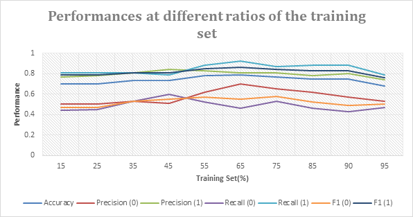
From the graph above, we can see that each metric reaches its summit when the ratio of the training set is between 0.45 and 0.75. Although the trend is not completely consistent, it shows an overall trend of first increasing and then decreasing. Four metrics (Accuracy, F1 (1), Recall (1), Precision (0)) are at their highest points when the ratio of the training set is 0.65, while F (0) and Recall (0) are at the local minimums. Moreover, at the ratio of 0.45, Precision (1) and Recall (0) reach their maximums, while Accuracy, Recall (1), F1 (1), and Precision (0) are at their local minimum values. Around the ratios of 0.35 and 0.50, the curves of Recall (1), F (1), and Precision (1) intersect at the same point, and Recall (0), F (0), and Precision (0) are roughly at the same level.

6. Discussion

Firstly, our experiment results are based on the parameters from restricted domains defined by us, and the domains are composed of several discrete values. Therefore, the results may not be globally optimized. To find global optimized parameters, more advanced mathematical skills are required.

Secondly, the evaluation standard for the best performance is defined by F1 score of negative instances, which is subjective and not a universal choice. Our concerns are based on the assumption that the financial institutions give priority to find people who are going to default in order to minimize the risk of default and avoid the loss on the asset. However, this assumption is not entirely true in reality. Therefore, the appropriate criteria will vary according to the macroeconomic background, regulatory environment and the risk preference of financial institutions. Financial institutions have the flexibility to adapt their assessment strategies to their own needs.

Thirdly, the result reveals that all metrics cannot meet their summits at the same ratio, and this phenomenon happens especially to two metrics, Recall (0) and Recall (1). When Recall (0) has its local minimums at ratios of 65% and 90%, Recall (1) has its local maximums, and Recall (1) reaches its local minimums when Recall (0) meets local max values at ratios of 45% and 75%. It is possible that this confrontation phenomenon comes from the RBF model’s preferences for different combinations of parameters. Furthermore, Recall (0) and Precision (0) have a tendency to diverge from each other. This trend makes logical sense. The more attempts the model makes to recall all negative instances, the more likely it is to make false judgments. Therefore, the rise of Recall (0) is partly at the expense of the decline of Precision (0).

7. Conclusion

We applied the SVM with RBF kernel on the South Germany credit dataset. And we tested different ratios of positive to negative instances with the optimized kernel function parameters in subjectively chosen domains to find the best performance. The result shows comparative improvements for different matrices when the ratio of positive to negative instances is relatively bigger and optimal parameters are applied. Also, we found that the ‘recall’ of the minority instance is relatively low, which means the model would be weak at detecting customers who are likely to default in practice. However, in the real financial world, the needs of institutions also change according to the macroeconomic background. Therefore, the model must make corresponding changes according to the actual demand.

References

[1]. Trivedi, S. K. (2020, September 28). A study on credit scoring modeling with different feature selection and machine learning approaches. Technology in Society. Retrieved December 24, 2021.
[2]. Wang, Y., Zhang, Y., Lu, Y., & Yu, X. (2020, July 27). A comparative assessment of Credit Risk Model based on machine learning --a case study of Bank Loan Data. Procedia Computer Science. Retrieved December 24, 2021.
[3]. Dastile, X., Celik, T., & Potsane, M. (2020, March 25). Statistical and Machine Learning Models in credit scoring: A systematic literature survey. Applied Soft Computing. Retrieved December 24, 2021.
[4]. Dumitrescu, E., Hué, S., Hurlin, C., & Tokpavi, S. (2021, June 29). Machine learning for credit scoring: Improving logistic regression with non-linear decision-tree effects. European Journal of Operational Research. Retrieved December 24, 2021.
[5]. Wu, C.-F., Huang, S.-C., Chiou, C.-C., & Wang, Y.-M. (2021, July 7). A predictive intelligence system of credit scoring based on deep multiple kernel learning. Applied Soft Computing. Retrieved December 24, 2021.
[6]. Tripathi, D., Edla, D. R., Kuppili, V., & Bablani, A. (2020, October 1). Evolutionary extreme learning machine with novel activation function for credit scoring. Engineering Applications of Artificial Intelligence. Retrieved December 24, 2021.
[7]. Zhang, W., Yang, D., Zhang, S., Ablanedo-Rosas, J. H., Wu, X., & Lou, Y. (2020, August 11). A novel multi-stage ensemble model with enhanced outlier adaptation for credit scoring. Expert Systems with Applications. Retrieved December 24, 2021.
[8]. Junior, L. M., Nardini, F. M., Renso, C., Trani, R., & Macedo, J. A. (2020, March 4). A novel approach to define the local region of dynamic selection techniques in imbalanced credit scoring problems. Expert Systems with Applications. Retrieved December 24, 2021.
[9]. Cortes, C., & Vapnik, V. (n.d.). Support-vector networks - machine learning. SpringerLink. Retrieved December 24, 2021.
[10]. Huang, Z., Chen, H., Hsu, C.-J., Chen, W.-H., & Wu, S. (2003, July 4). Credit rating analysis with support Vector Machines and neural networks: A market comparative study. Decision Support Systems. Retrieved December 24, 2021.
[11]. Min, J. H., & Lee, Y.-C. (2007, September 12). A practical approach to credit scoring. Expert Systems with Applications. Retrieved December 24, 2021.
[12]. Chen, C.-C., & Li, S.-T. (2014, June 12). Credit rating with a monotonicity-constrained support vector machine model. Expert Systems with Applications. Retrieved December 24, 2021.
[13]. Jiang, H., Ching, W.-K., Yiu, K. F. C., & Qiu, Y. (2018, July 10). Stationary mahalanobis kernel SVM for Credit Risk Evaluation. Applied Soft Computing. Retrieved December 24, 2021.
[14]. Z. Dai, Z. Yuchen, A. Li and G. Qian, (2021, April 02) The application of machine learning in bank credit rating prediction and risk assessment, 2021 IEEE 2nd International Conference on Big Data, Artificial Intelligence and Internet of Things Engineering, from https://ieeexplore.ieee.org/document/9389901
[15]. Yeh, I.-C., & Lien, C.-hui. (2008, January 14). The comparisons of data mining techniques for the predictive accuracy of probability of default of credit card clients. Expert Systems with Applications. Retrieved December 24, 2021.
Cite this article
Lei,L.;Liu,X. (2023). Support Vector Machine for Credit System: The Effect of Parameter Optimization and Training Sample. Theoretical and Natural Science,2,113-120.
Data availability
The datasets used and/or analyzed during the current study will be available from the authors upon reasonable request.
Disclaimer/Publisher's Note
The statements, opinions and data contained in all publications are solely those of the individual author(s) and contributor(s) and not of EWA Publishing and/or the editor(s). EWA Publishing and/or the editor(s) disclaim responsibility for any injury to people or property resulting from any ideas, methods, instructions or products referred to in the content.
About volume
Volume title: Proceedings of the International Conference on Computing Innovation and Applied Physics (CONF-CIAP 2022)
© 2024 by the author(s). Licensee EWA Publishing, Oxford, UK. This article is an open access article distributed under the terms and
conditions of the Creative Commons Attribution (CC BY) license. Authors who
publish this series agree to the following terms:
1. Authors retain copyright and grant the series right of first publication with the work simultaneously licensed under a Creative Commons
Attribution License that allows others to share the work with an acknowledgment of the work's authorship and initial publication in this
series.
2. Authors are able to enter into separate, additional contractual arrangements for the non-exclusive distribution of the series's published
version of the work (e.g., post it to an institutional repository or publish it in a book), with an acknowledgment of its initial
publication in this series.
3. Authors are permitted and encouraged to post their work online (e.g., in institutional repositories or on their website) prior to and
during the submission process, as it can lead to productive exchanges, as well as earlier and greater citation of published work (See
Open access policy for details).