1. Introduction

The National Basketball Association (NBA) is one of the most successful league which attract most of skillful players around world. The team from League will sign contract with high amount of money, some unreasonable contract will lead to low profit for the NBA and will cause losses [1]. Stephen Curry in the Golden State Warriors has earned at least $51.9 million in the 2023-2024 season, and Lebron James in the Los Angles Lakers has earned $51.42 million [2]. In order to solve this problem, the league has introduced a new policy called “salary cap” which limit the maximum on the expenditure of each team [3]. Since each team have this kind of restriction, team chiefs should consider how to make effective contacts with players for rational allocation of limited budget. It’s very important for regulator of each team to analyse player’ salaries taking into account different factors that represent the performance of each players [4].

The field of analysis of player salary is under-researched, there is a lack of research applying machine learning model in this area. Chen tried to construct a linear regression model to analyse the relationship between players’ salary and field data [5]. Özbalta et al. found the distribution of each factors including positions and points per games against their salaries and got the correlation coefficient of different field data and found that the shooting efficiency and defence ability have a significant impact on the players’ salaries [6]. Kremer also constructed a multiple linear regression to analyse the correlation among ages, career prospective and overall ability of players, in order to predict their salaries. The final result indicated that the overall ability has a strong correlation with salary [7]. In NBA, there are many factors which affect the salary including but not limited points per game, number of assists and blocks. Therefore, this paper only focused on factors which contribute the effect on final salary and presents the examination of potential variables to establish a multiple regression model to analyse salary of players [8]. In 2022, Papadaki and Tsagris used different data including roster competition, defensive contributions, and impact of bench players by Player Impact Estimate (PIE) to predict future performance to forecast salaries with average positional production [9]. Zhang found the relation between salary and field data of players by constructing a multiple statistics model, they calculated the value of ordinary least squares (OLS) and the difference between predicted value and true value [8].

In this paper, the previous approached has been summarized and applied to predict players’ salaries. This paper divide into three parts including data preprocessing which normalizing data to make them useful, and constructing a multiple linear regression model which salary is dependent variable and filed data including age, scoring, boarding and assisting as independent variable. Using the result to provide conclusion for guiding idea for team managers in future work [10]. The structure of work has been introduced as follow. Section 2 describes the methods used in this paper, and compare each variables strengths and weakness. The final section provides the conclusion and guiding suggestions.

2. Methodology

2.1. Data source and description

In order to make sure that the utility and accuracy of datasets, the data use in this paper come from the Kaggle. Kaggle is an authoritative website which contain many different types of datasets provided by users. Many researchers including professors, students in university and other academic staffs will use the datasets and models provided by Kaggle to conduct research in analysis of datasets and work out the results.

The datasets chosen from the Kaggle is consist of the most crucial statistics in players' career which is from 2023-2024 seasons including their salaries, scoring, assist, name and positions. The indicators that this paper used all have considerable impacts on players' salaries.

2.2. Method introduction

The salaries of players act as the dependent variables and the field data is dependent variable, the linear regression function will be used for analysis. Here is the linear function.

\( E(Y)={β_{0}}+{β_{1}}{x_{1}}+{β_{2}}{x_{2}}+⋯+{β_{13}}{x_{12}}+e \) (1)

Where \( {x_{i}} \) represent the value of each fielded data and \( Y \) represent salary of player's salary. \( {β_{i}} \) represents the regression coefficient which indicate the effect of each data on final outcomes. \( e \) shows the error variable.

3. Results and discussion

3.1. Descriptive analysis

In order to acquire a clear and reliable datasets of each statistic of players, the descriptive statistical analysis is conducted on these data. There were various scatter graphs that indicating the relationship between each variable against salaries each players received. Figure 1 indicates the relationship between age and salaries.

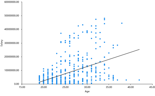
Figure 1. Scatterplot of age and salary.

Figure 1 indicates the linear correlation between the salary of the players and their age. The conclusion can be drawn from this graph that there are no significant relations between these two types of variables, but it demonstrates the higher payments are concentrated on the ages between 30 to 35 with some extra at around 40. The next relation showed in Figure 2 indicates the linear regression between salary and number of game played by players.

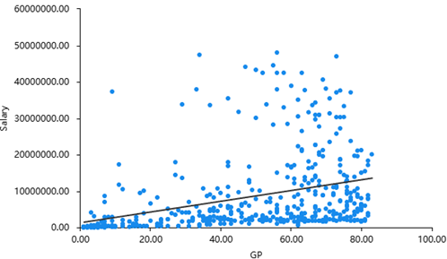
Figure 2. Scatterplot of GP and salary.

Figure 2 indicates that there is a clear correlation between the salary and the number of game played by each player, most of players with 40 games to 60 games tend to receive the higher salaries than the players at the rest of ages. Relationship between the minutes played and the salaries is indicated by the Figure 3 below.

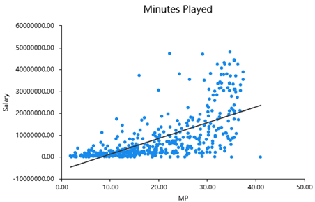
Figure 3. Scatterplot of MP and salary.

There is a strong positive correlation between the minutes played by each player and the salaries received. Players have higher minutes played tend to receive higher salaries than those with lower minutes played. Figure 3 shows that players with time at the field around 25 to 35 minutes receive higher wages, with the highest paid players at around 35 minutes. The final Figure 4 shows that the relations between the player salaries against the points that each player gained in each game.

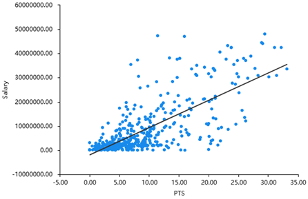
Figure 4. Scatterplot of PTS and salary.

There is a significantly strong relations between the salaries and points per game, with the trend that higher points gained, the more money players received. Figure 4 indicates that players with points between 25 to 35 tend to receive a higher salary than those with only 0 to 10 points.

Furthermore, there is another diagram showing the distribution of salaries against each player. This diagram indicates there is a really huge range among the players’ salaries. Stephen Curry is a players received the highest payment which is about 55.76 million dollars and is the only wages that beyond 50 million dollars. There are more than 75 percent players received the salaries lower than 25 million dollars with only a few of players received the salaries about more than 40 million. There are approximately 300 players earn about 25 million to 35 million dollars, which have a large difference compared with the top salaries in the association.

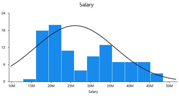
Figure 5. Distribution of salary.

Apart from that, there is another diagram (Figure 5) that indicates the distribution of salaries gained by each worker. The figure shown the distribution of salaries against the positions that each players played.

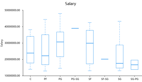
Figure 6. Boxplot of salary by position.

As indicated in Figure 6, there is no significant difference in each position. Point guard tend to obtain higher salaries than the other positions, it has the higher average salaries than the other positions as well. The point guard own an outstanding players called Stephen Curry which received the highest salaries.

The next diagram showed one of the significant factor age which has a considerable influence on players’ salaries. This diagram indicates that 31 to 33 tend to obtain the higher average salaries than other players at other ages due to the players often keep the peak state during these periods. Players at 35 to 38 often receive a lower salary compared with the ages between 31 to 33 and the ages between 23 to 27 receive a lower average salary as well. However, there is a exception which receive a very high salaries, that is Lebron James receiving salaries about more than 40 million dollars. This is because he kept his outstanding performance on the field and his very high business values he brought to the League and his team. There are some players at 24 to 29 received really high ages, this is because the players at these ages tend to have low ability and lack enough experience, they need more time to develop their own skills, experience and business values to increase the amount of their salaries (Figure 7).

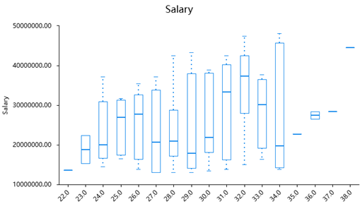
Figure 7. Boxplot of salary by age.

3.2. Model results

The detailed relations between the salaries of each player and some of the field data performed by each player have been conducted by constructing a linear regression model. In the table 1 below, standard error and B indicates the coefficient values, and beta is the coefficient value when there is a situation that when constant is zero. The t and p below show the significance of each of each variable and can be used to calculate the value of its statistical significance. The value covariance can be obtained by the value of tolerance and VIF. The table indicates the R squared value is 0.665 which shows that these variables can contribute the 66.5 percent on players’ salaries.

Table 1. Model results.

Remark:Dependent Variable = Salary

* p<0.05 ** p<0.01

4. Conclusion

This research focuses on examining the relationship between basketball players’ performance metrics on the court and their salary compensation, with the goal of predicting teams’ salary cap management and players’ future earnings. By utilizing data from the 2022-2023 NBA season, regression analyses were carried out with per-game statistics as the independent variables and player salaries as the dependent variable. Descriptive statistics and linear regression revealed issues with multicollinearity among the independent variables, contrary to the findings from graphical representations that illustrated the relationship between player salaries and performance metrics. According to these graphical analyses, shooting efficiency (such as PTS, 3PA, 2PA) and defensive capabilities (such as REB, STL, BLK) were found to have a substantial influence on player salaries.

References

[1]. Zhang M 2024 Analysis of NBA Player Salary using Linear Regression Analysis. Highlights in Science, Engineering and Technology, 88, 509-515.
[2]. Feng X, Wang Y and Xiong T 2023 NBA Player Salary Analysis based on Multivariate Regression Analysis. Highlights in Science, Engineering and Technology, 49, 157-166.
[3]. Chen X, Lin H, Pang L, et al. 2023 A Survey of Forecasting the Salary for Players in National Basketball Association. Journal of Education, Humanities and Social Sciences, 16, 1-6.
[4]. Zhao Y 2022 Model Prediction of Factors Influencing NBA Players’ Salaries Based on Multiple Linear Regression. 2022 2nd International Conference on Economic Development and Business Culture (ICEDBC 2022). Atlantis Press, 1439-1445.
[5]. Chen S 2016 Model Prediction of Factors Influencing NBA Players' Salaries Based on Multiple Linear Regression. Business, 26, 1.
[6]. Özbalta E, Yavuz M and Kaya T 2022 National Basketball Association Player Salary Prediction Using Supervised Machine Learning Methods. Intelligent and Fuzzy Techniques for Emerging Conditions and Digital Transformation: Proceedings of the INFUS 2021 Conference, 24-26.
[7]. Kremer P 2019 Predicting if NBA Teams Will Make the Playoffs Based on Estimated Wins Added (EWA) and Salary. Utica College.
[8]. Zhang J 2024 National Basketball Association Salary Prediction: A Data-Driven Linear Regression Analysis. Highlights in Business, Economics and Management, 24, 1059-1064.
[9]. Papadaki I and Tsagris M 2022 Are NBA Players’ Salaries in Accordance with Their Performance on Court. Advances in Econometrics, Operational Research, Data Science and Actuarial Studies: Techniques and Theories. Cham: Springer International Publishing, 405-428.
[10]. Swanson A 2015 How we provoked the wrath of some of the world's most perfect people. Washington Post, 10.
Cite this article
Xiong,A. (2024). Analysis of NBA player salary based on multiple linear regression model. Theoretical and Natural Science,51,206-213.
Data availability
The datasets used and/or analyzed during the current study will be available from the authors upon reasonable request.
Disclaimer/Publisher's Note
The statements, opinions and data contained in all publications are solely those of the individual author(s) and contributor(s) and not of EWA Publishing and/or the editor(s). EWA Publishing and/or the editor(s) disclaim responsibility for any injury to people or property resulting from any ideas, methods, instructions or products referred to in the content.
About volume
Volume title: Proceedings of CONF-MPCS 2024 Workshop: Quantum Machine Learning: Bridging Quantum Physics and Computational Simulations
© 2024 by the author(s). Licensee EWA Publishing, Oxford, UK. This article is an open access article distributed under the terms and
conditions of the Creative Commons Attribution (CC BY) license. Authors who
publish this series agree to the following terms:
1. Authors retain copyright and grant the series right of first publication with the work simultaneously licensed under a Creative Commons
Attribution License that allows others to share the work with an acknowledgment of the work's authorship and initial publication in this
series.
2. Authors are able to enter into separate, additional contractual arrangements for the non-exclusive distribution of the series's published
version of the work (e.g., post it to an institutional repository or publish it in a book), with an acknowledgment of its initial
publication in this series.
3. Authors are permitted and encouraged to post their work online (e.g., in institutional repositories or on their website) prior to and
during the submission process, as it can lead to productive exchanges, as well as earlier and greater citation of published work (See
Open access policy for details).