1. Introduction

Forecasting stock prices is a crucial and popular topic within data science, significantly benefiting investors, traders, analysts, and financial institutions. Time Series Forecasting (TSF) has made significant headway due to the growing availability of historical data and the growing need for production forecasting [1]. Traditional forecasting methods often face limitations such as complexity and time consumption.

A time series consists of a sequence of well-defined data points collected at regular intervals over time. Analysing time series data is a fundamental component of statistics, aiming to identify characteristics within the data set and project future values based on these features [2]. However, time series analysis frequently encounters difficulties due to dynamic economic conditions. Thus, finding effective methods for time series analysis is essential for improving forecasting accuracy and efficiency.

Regression models are a common approach to addressing these challenges. Different forecasting models can work better together to capture data trends, and theoretical and empirical research have demonstrated that a mix of forecasts frequently performs better than individual models [3]. Among various regression models, the Auto-Regressive Integrated Moving Average (ARIMA) model, an enhancement of the ARMA model, is particularly efficient for predicting time series data, including stock prices. The ARIMA model requires only historical data to generate forecasts, allowing it to improve accuracy while minimizing the number of parameters [4]. Additionally, ARIMA models have proven to be excellent for short-term forecasting due to the slower change of short-term factors [5].

This paper will explain how the ARIMA model works and demonstrate its application in forecasting Microsoft's stock price from 1987 to 2024. This paper will begin by introducing the dataset and the ARIMA model. The dataset will then be divided into training sets and test set, with the goal of building a suitable ARIMAX model for the training set and assessing accuracy using the test set. Finally, this paper will discuss potential improvements to the model and provide recommendations for future applications of the ARIMA model.

2. Methodology

2.1. Data source

This dataset shows the stock price of Microsoft from 1987 to 2024. The data set contains 7 daily columns. This paper will focus on dates and 2 variables (Closing Price and Adjusted Closing Price): The Closing Price is the price at which a security is transacted for the last time before the market closes for regular business. An adjustment to a stock's closing price by calculation is called an adjusted closing price. Due to its inability to take into account potential price-moving factors, the initial closing price may not represent the most accurate assessment of the stock or asset. The price modifications that must be made will therefore be included in the modified closing price (Figure 1).

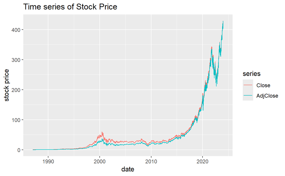
Figure 1. The time plot of Closing Prices (red) and Adjusted Closing Prices (blue)

Figure 1 shows the time plot of Closing Prices and Adjusted Closing Prices of Microsoft Stock. Both time series have an increasing trend and the speed of increasing also increases with time. So, it is very obvious to see that these patterns fit an exponential growth except the stock price around 2022, they have a great falling suddenly and come back to an increasing trend after about one year. Compare with the bule line, values of the red line are a bit larger especially around 2000.

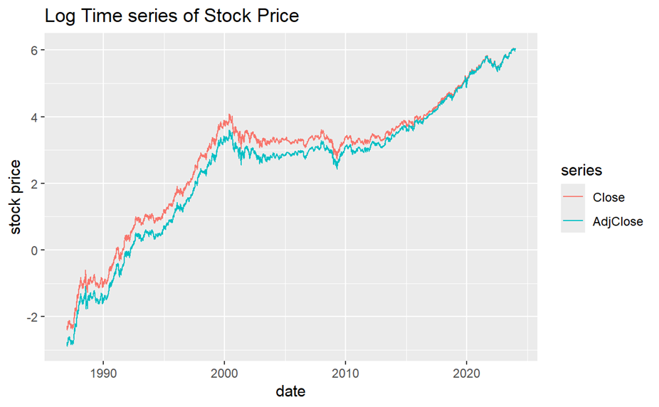
Figure 2. The log time plot of Closing Prices (red) and Adjusted Closing Prices (blue)

Figure 2 shows the log time plot of Closing Prices and Adjusted Closing Prices of Microsoft Stock. In log version, the plot shows more details than the origin one. These time series still have an increasing trend but the speed of increasing is like a linear trend. As a result, the exponential growth of 2 lines in Figure 1 is proved by the linear trend of their log version plots. Also, the difference between 2 lines is more obvious in this plot than Figure 1. The red line is higher than the blue line and 2 lines become more and more similar by 2015. Combine with these 2 plots, adjustments decrease values of Closing Price in order to accurate the valuation of stock.

2.2. Autocorrelation of time series

The following Autocorrelation Function (ACF) plot is created to see more the properties of time series.

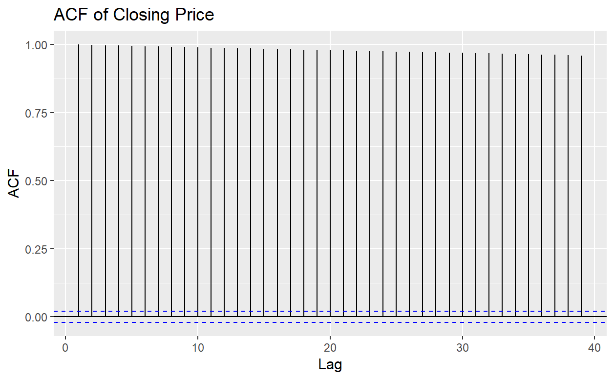
Figure 3. The ACF plot of Closing Prices

Figure 3 shows the ACF plot of Closing Price. The autocorrelations are very close to 1, this means there is a strong linear relationship among lagged values of Closing Prices time series.

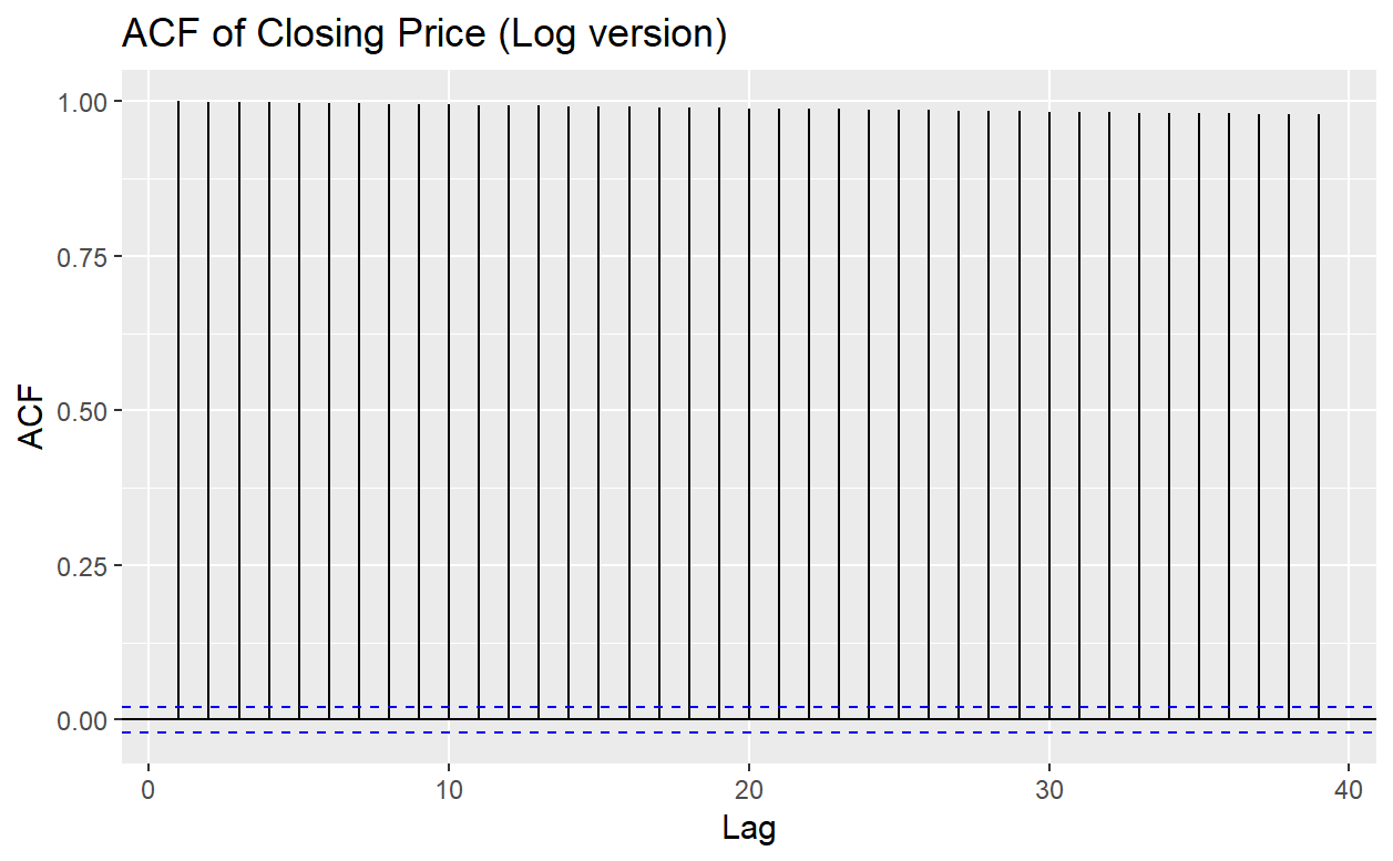
Figure 4. The ACF plot of Closing Prices (log version)

Figure 4 shows the ACF of log version of the Closing Prices time plot. In this plot, the autocorrelations are still very close to 1, take log to values cannot decrease the autocorrelation for this time series but there is still a little difference between Figure 3 and 4. So there might be some influences if taking log to values of time series. From the definition of the autocorrelation, there will not be any obvious changes if taking log to values of time series.

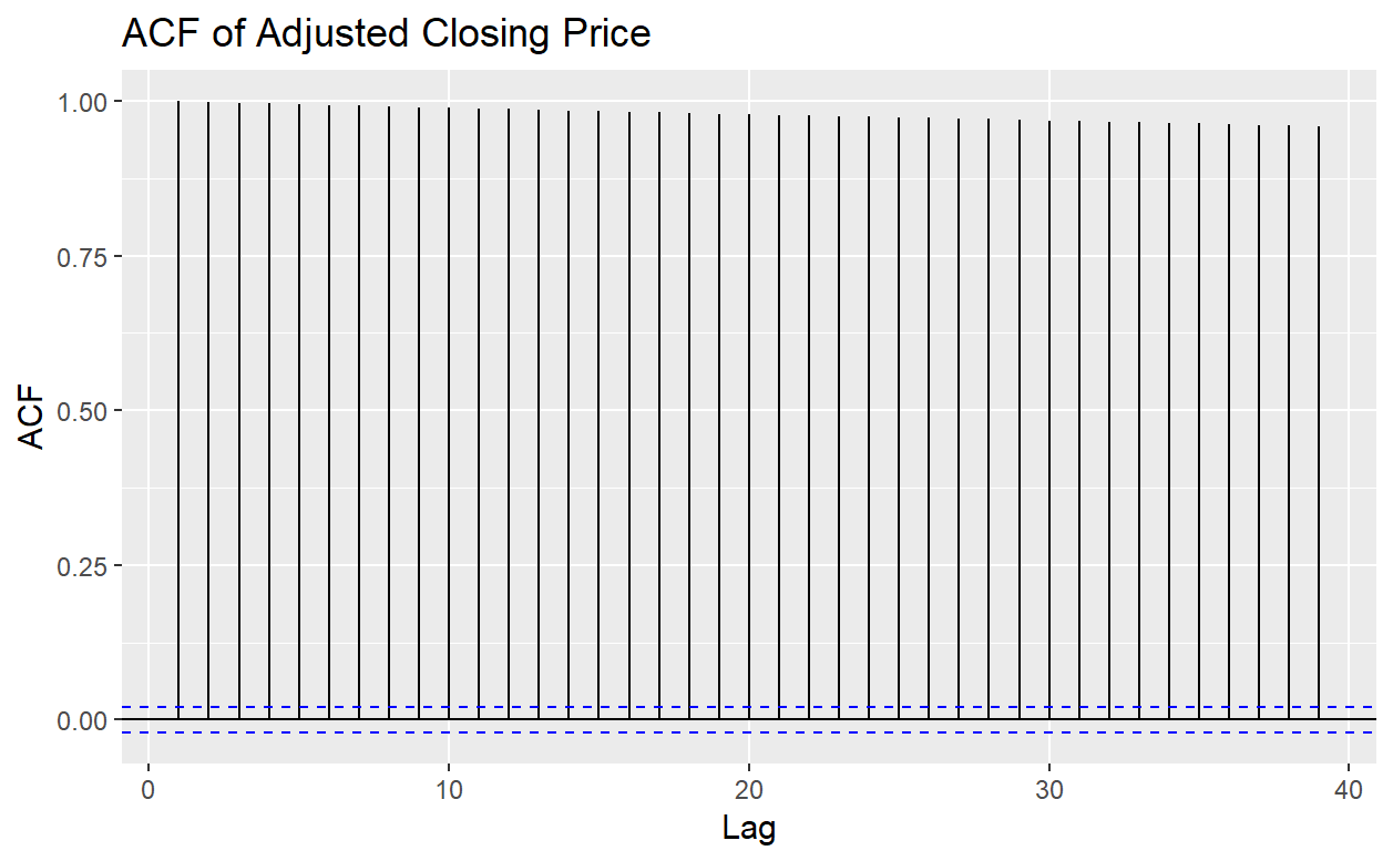
Figure 5. The ACF plot of Adjusted Closing Prices

Figure 5 shows the ACF plot of Adjusted Closing Price. Similar to Figure 3, the autocorrelations after adjustments are still very close to 1, so the lagged values of Adjusted Closing Prices time series also have a strong linear relationship.

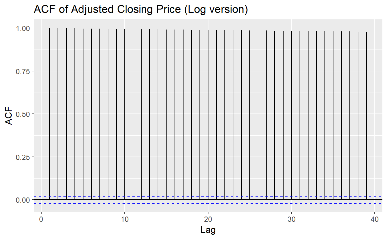
Figure 6. The ACF plot of Adjusted Closing Prices (log version)

Figure 6 shows the ACF of log version of the Adjusted Closing Prices time plot. This plot also gives evidence that taking log to values cannot decrease the autocorrelation since the autocorrelation represents the trend and period of a time series. However, taking log values is a specific method for exponential growth data, so it produces little changes on autocorrelations.

2.3. Introduction of ARIMA model

Since linear models are easy to understand and use, academics have focused a lot of their attention on them over the last few decades [6]. The most popular linear technique in financial forecasting is the ARIMA model, which has demonstrated effective short-term forecasting capabilities [7]. The process of determining, fitting, and validating ARIMA models using time series is called the Box-Jenkins methodology [8]. The ARIMA model has four parts: Autoregressive (AR), Integrated (I) and Moving Average (MA). The ARIMAX model is mathematically represented as:

\( y_{t}^{ \prime }=\sum _{i=1}^{p}{ϕ_{i}}{y \prime _{t-i}}+\sum _{j=1}^{q}{θ_{j}}{y \prime _{t-j}}+{ε_{t}}+c \) (1)

Where: t: time. \( {y_{t}} \) : target variable at time t. \( {y \prime _{t}}={{(1-B)^{d}}y_{t}} \) : target variable after differencing. c: constant term. \( {ϕ_{i}} \) : AR coefficients. \( {θ_{j}} \) : MA coefficients. \( {ϵ_{t}} \) : white noise error term. B: backward shift operator and \( {By_{t}}={y_{t-1}} \) . The order of (AR, I, MA) is (p,d,q).

3. Results and discussion

3.1. Dividing data set

From the log time series plot (Figure 2), the data set can be divided into 3 parts for training: 1987-2000, This part has an obvious increasing trend with a large slope (P1). 2000-2010: Time series become stable and did not have any trend in this part (P2). 2010-2020: In this part, stock prices begin to increase again but slope is not a constant (P3). At last, data from 2020 to 2024 are used for testing.

3.2. Model results

Finding the best p,d,q combination by choosing the smallest AIC value. Table 1 shows the ARIMA coefficients of model1 (the best ARIMA model with log values of Adjusted Closing Prices from 1987 to 2000). Here the (p,d,q) combinations are (4,1,1).

Table 1. ARIMA coefficients of model 1

For model 2 (the best ARIMA model with log values of Adjusted Closing Prices from 2000 to 2010) the best (p,d,q) combinations are (0,1,0). That means this time series only need to have a differencing of order 1, it does not have AR and MA parts.

Table 2. ARIMA coefficients of model3

Table 2 shows the ARIMA coefficients of model3 (the best ARIMA model with log values of Adjusted Closing Prices from 2010 to 2020). Here the (p,d,q) combinations are (1,1,1).

The 3 models are produced by different time periods, model 2 is the simplest one since the time series from 2000 to 2010 is the smoothest. Also, model1 has the largest order since its time series has the highest growing speed.

3.3. Checking accuracy of 3 models

Table 3 shows the AIC, AICc and BIC values of 3 models. From values of AIC, AICc and BIC, model1 have a higher accuracy than other 2 models since all values of model1 are less than that of model2 and model 3.

Table 3. Comparison of accuracy of 3 models

\( AIC = (- 2) log maximum likelihood + 2 (number of parameters) \) , where log represents a natural logarithm, is a measure of how poorly a model fits data defined using the maximum likelihood technique [9, 10].

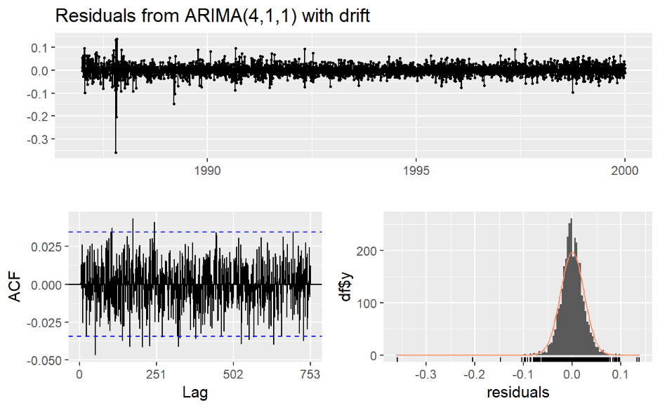
Figure 7. The residual plot of model 1

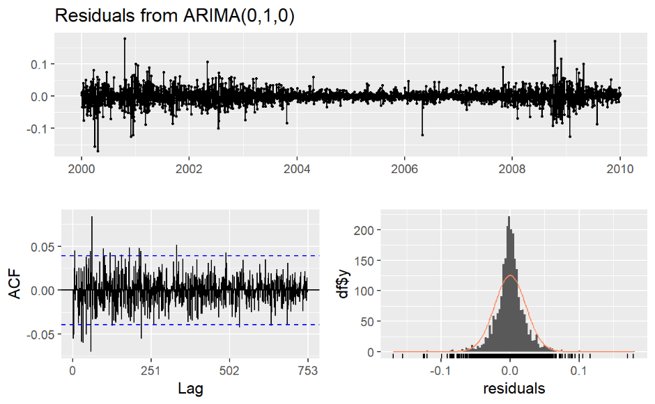
Figure 8. The residual plot of model 2

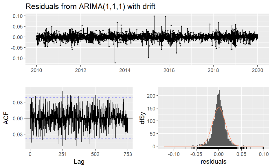
Figure 9. The residual plot of model 3

Figure 7, 8, 9 show residual plots of model 1, 2, 3 separately. From these plots, residuals of all 3 models are around 0 and autocorrelations are white noise from p values of them (see table 4 below). Also, the residuals of them are very approaching to a normal distribution.

Table 4. P values of 3 models

4. Models forecasting

4.1. Forecasting from 2020 to 2024

Figure 10 gives a prediction of log Adjusted Closing Prices of Microsoft Stock from 2020 to 2024. Figure 11 shows the log time plot of Adjusted Closing Prices of Microsoft Stock from 2020 to 2024. Compare with these two figures, model3 gives a good forecasting. In both plots, log stock prices have an increasing trend and vary in range of (5, 6).

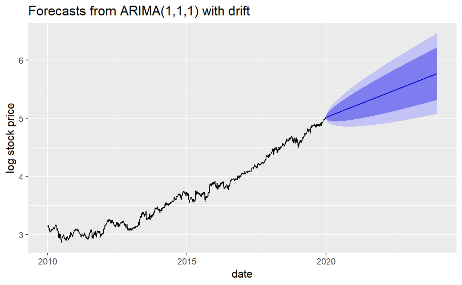
Figure 10. The forecasting plot of model 3

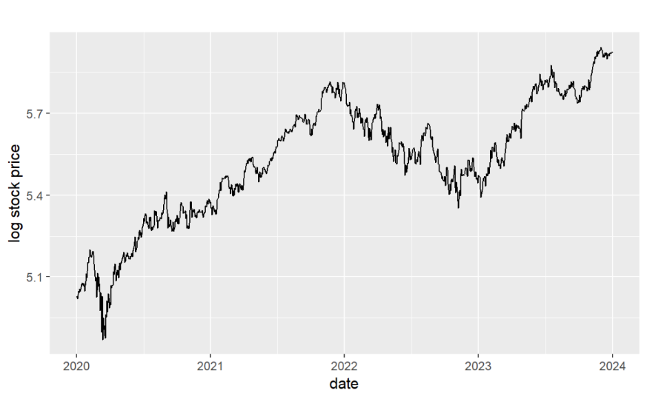
Figure 11. The time plot of Adjusted Closing Prices (log version) from 2020 to 2024

4.2. Forecasting in the future 2 years

Figure 12 gives a prediction of log Adjusted Closing Prices of Microsoft Stock from 2024-05 to 2026-05. From the plot, stock prices still have an exponential increasing trend and real values of stock prices will reach 600 in 2026, the values will vary in range of (400, 1100).

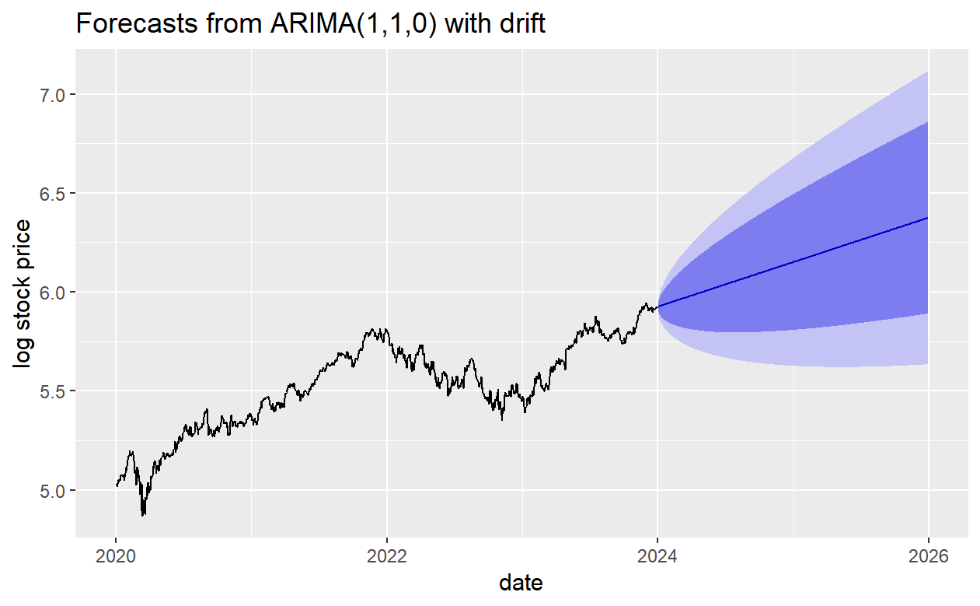
Figure 12. The predicting Adjusted Closing Stock Prices in the future 2 years (log version)

5. Conclusion

Generally, the ARIMA model does well in the stock price forecasting but it still needs some improvements if people want to apply it in their real lives. The ARIMA model is very suitable for short term data but not long term. Since it is difficult to capture accurate changes in instances of abrupt changes in the data set (when the variance is considerable), changes in government policies, economic instability (structural break), etc., this model becomes unreliable for forecasting in this scenario. The log version of time series is necessary for forecasting stock prices especially in this paper since ARIMA model is a linear regression model and the Microsoft Stock Prices have an exponential growing trend. Taking log to values of time series can make the slop become linear and smooth. For other stock prices log version may help decrease complicity and show more details of the data set. At last, although the ARIMA model has some disadvantages on predicting stock price, it is very useful on financial forecasting especially for data sets which can be approximate to linear combinations. Wish the results and advice in this paper can help investors.

References

[1]. Khan S and Alghulaiakh H 2020 ARIMA model for accurate time series stocks forecasting. International Journal of Advanced Computer Science and Applications, 11(7).
[2]. Mondal P, Shit L and Goswami S 2014 Study of effectiveness of time series modeling (ARIMA) in forecasting stock prices. International Journal of Computer Science, Engineering and Applications, 4(2), 13.
[3]. Pai P F and Lin C S 2005 A hybrid ARIMA and support vector machines model in stock price forecasting. Omega, 33(6), 497-505.
[4]. Wadi S A L, et al. 2018 Predicting closed price time series data using ARIMA Model. Modern Applied Science, 12(11), 181-185.
[5]. Tse R Y C 1997 An application of the ARIMA model to real‐estate prices in Hong Kong. Journal of Property Finance, 8(2), 152-163.
[6]. Fattah J, Ezzine L, Aman Z, et al. 2018 Forecasting of demand using ARIMA model. International Journal of Engineering Business Management, 10.
[7]. Ariyo A A, Adewumi A O and Ayo C K 2014 Stock price prediction using the ARIMA model[C]//2014 UKSim-AMSS 16th international conference on computer modelling and simulation. IEEE, 106-112.
[8]. Nochai R and Nochai T 2006 ARIMA model for forecasting oil palm price. Proceedings of the 2nd IMT-GT Regional Conference on Mathematics, Statistics and applications. Penang: Academia, 13-15.
[9]. Akaike H 1987 Factor analysis and AIC. Psychometrika, 52, 317-332.
[10]. Guha B and Bandyopadhyay G 2016 Gold price forecasting using ARIMA model. Journal of Advanced Management Science, 4(2).
Cite this article
Ma,H. (2024). Using ARIMA Model to Forecast the Stock Price of Microsoft. Theoretical and Natural Science,42,135-144.
Data availability
The datasets used and/or analyzed during the current study will be available from the authors upon reasonable request.
Disclaimer/Publisher's Note
The statements, opinions and data contained in all publications are solely those of the individual author(s) and contributor(s) and not of EWA Publishing and/or the editor(s). EWA Publishing and/or the editor(s) disclaim responsibility for any injury to people or property resulting from any ideas, methods, instructions or products referred to in the content.
About volume
Volume title: Proceedings of the 2nd International Conference on Mathematical Physics and Computational Simulation
© 2024 by the author(s). Licensee EWA Publishing, Oxford, UK. This article is an open access article distributed under the terms and
conditions of the Creative Commons Attribution (CC BY) license. Authors who
publish this series agree to the following terms:
1. Authors retain copyright and grant the series right of first publication with the work simultaneously licensed under a Creative Commons
Attribution License that allows others to share the work with an acknowledgment of the work's authorship and initial publication in this
series.
2. Authors are able to enter into separate, additional contractual arrangements for the non-exclusive distribution of the series's published
version of the work (e.g., post it to an institutional repository or publish it in a book), with an acknowledgment of its initial
publication in this series.
3. Authors are permitted and encouraged to post their work online (e.g., in institutional repositories or on their website) prior to and
during the submission process, as it can lead to productive exchanges, as well as earlier and greater citation of published work (See
Open access policy for details).