1. Introduction

In recent years, it is widely known that video has a great influence on many aspects of our lives, including television, games, scientific research, and so on. Although video is of great importance to us, it is a pity that the video is always contaminated by noise, which can lower the quality of the video and disturb the usage of the video. In this case, no matter whether for the quality of life or for the advance of technology, we should eliminate the noise. Therefore, the research on effective video filtering methods which can significantly reduce the noise in the video is necessary without a doubt. Currently, most of the video noise follows the Gaussian distribution [1]. Consequently, the main objective of research into video filtering is to decrease the effect of Gaussian noise as much as possible with the premise of containing the video image.

There have been two main varieties of the existing video filtering methods [2-6]. Firstly, the traditional video denoising approach is spatial image filtering and a typical approach within this category is bilateral filtering. In [2], Gavaskar et al. mentioned a fast adaptive bilateral filtering algorithm whose complexity will not be dependent on the spatial filter width. It is on the basis of the finding that they can exploit the appropriately defined local histogram to perform the concerned denoising in range space. Particularly, through matching the moments of the multinomial with those of the target histogram to fit the multinomial, and then utilizing integration-by-parts to recursively calculate the analytic function, the brute-force implementation had been dramatically developed without obvious distortions in the visual quality. Similarly, another fast bilateral filtering method [3] was proposed by Papari et al., which served for huge 3D images. The approach extended the bilateral filter kernel to the sum of decomposed factors. Thus, the bilateral filter was simplified into several Gaussian convolutions, whose computational speed was ten times more than the normal bilateral filter. Secondly, the other main denoising method scheme is the spatial-temporal filter that considers the temporal information except for spatial. A classical model was a Multi-Hypothesis motion compensated filter(MHMCF) [4]. MHMCF employed several assumptions including temporal predictions to evaluate the pixel that was contaminated with noise. Based on MHMCF, Guo issued a quick filtering approach FMHMCF [5], and FMHMCF can find trustworthy hypotheses through edge-preserved low-pass prefiltering and noise-robust fast multi-hypothesis search when only confirming a few positions. As a result, the filtering speed was obviously faster than before. Besides, according to [6], a denoising algorithm was mentioned which was based on the spatial wiener filter and the temporal filter. On the basis of the image feature and noise level, it can adjust the filter mask adaptively. The advantage of this method was that it could maintain the image feature more complete and it was simple to implement.

However, although these approaches can get effective filtering results, there are few methods denoising based on the human visual system (HVS) characteristics. Moreover, it is unavoidable that the noise from some of the filtered pixels can be still perceived by our eyes or a number of the pixels can be distorted due to the excessive filtering. Consequently, we propose a perception-oriented spatial-temporal video filtering algorithm by taking the HVS into consideration to improve the perceptual filtering performance. The method is divided into two steps. Firstly, we design an adaptively block-level bilateral filtering algorithm with spatial-temporal consideration. The filter strength is adaptively adjusted depending on the difference between the original and motion compensation blocks. Secondly, the just noticeable difference (JND) perceptual model [7] which indicated the perceptual characteristics for each pixel of HVS was introduced to further adjust the filter strength. Through these two steps, we can effectively conduct perceptual filtering to achieve better subjective performance. The experimental results show that the proposed algorithm obtained remarkable performance improvement by PSNR and PSPNR with 46.13dB and 54.72dB, respectively. Additionally, brilliant filtering quality is also achieved by subjective filtering image comparison.

The remainder of the paper is organized as follows: Section 2 will describe the bilateral filtering algorithm on the basis of motion estimation (ME). The video denoising method which is based on JND will be introduced in Section 3, followed by experiment and conclusion in Section 4, and Section 5, respectively.

2. The combination of ME and bilateral filtering

In this part, we will first describe the bilateral filtering, followed by ME and the proposed spatial-temporal filtering algorithm without JND, and the final perceptual filtering method will be mentioned later.

2.1. Bilateral filtering

Bilateral filtering is a kind of image denoising approach, which removes the noise while maintaining the edge information. It is a nonlinearity filtering method [8] that is applied extensively in the field of image processing, especially when we need to keep the edge details. A bilateral filter combines the characteristics of a gaussian filter and an edge-preserving filter. Consequently, the weighted average is performed by considering two factors: spatial proximity and pixel value similarity. Certainly, the weight is divided into two varieties: for the spatial proximity, the closer the distance is, the greater the weight is. For the pixel value similarity, the more similar the value is, the greater the weight is. Let I ̂_(i,j) be the value of the output pixel which is located at (i ,j), so that it is determined by a weighted average of the pixel values in the neighborhood of (i ,j),

\( {\hat{I}_{i,j}}= \frac{\sum _{y=-3}^{3}\sum _{x=-3}^{3}{I_{x,y}}{w_{x,y}}}{\sum _{y=-3}^{3}\sum _{x=-3}^{3}{w_{,x,y}}} \) , (1)

where \( (x,y) \) is the neighborhood index of \( (i , j) \) , and \( {I_{x,y}} \) is the value of the pixel in \( (x,y) \) . \( {w_{x,y}} \) is the weight of \( (x,y) \) when calculating the filtered value of position \( (i , j) \) , it is the product of spatial weight and similarity weight,

\( {w_{x,y}} ={w_{s}}*{w_{r}} \) , (2)

where the spatial weight is calculated as,

\( {w_{s}}=exp{(-\frac{{(i-x)^{2}}+{(j-y)^{2}}}{2{sigm{a_{s}}^{2}}})} \) , (3)

while the similarity weight is given as,

\( {w_{r}}=exp{(-\frac{{|{I_{i,j}}-{I_{x,y}}|^{2}}}{{2sigm{a_{r}}^{2}}})}, \) (4)

where \( {I_{i,j}} \) is the value of the pixel in \( (i , j) \) , \( sigm{a_{s}} \) is the intensity of spatial and \( sigm{a_{r}} \) is the intensity of similarity, respectively.

2.2. Motion estimation

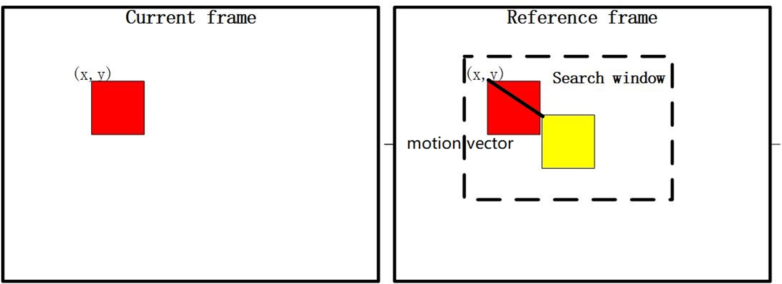
Figure 1. The process of motion estimation

ME is a crucial technology in the field of video processing, which aims to predict the motion of objects in the scene by analyzing the changes between consecutive video frames [9]. The principle of ME is to estimate the motion displacement of two serial frames as shown in figure 1, followed by motion compensation which is to align the images based on the motion displacement. The common matching criterion in ME is SAD (Sum of Absolute Difference) as computed as,

\( SAD= \sum _{j=0}^{B}\sum _{i=0}^{B}|{{I_{c}}_{i,j}}-{{I_{R}}_{i,j}}| \) , (5)

where \( B \) is the size of the block, \( {{I_{c}}_{i,j}} \) is the value of the current pixel at \( (i,j) \) , and \( {{I_{R}}_{i,j}} \) is the value of the reference pixel at \( (i,j) \) . The smaller the \( SAD \) is, the better match block can be found to the original one, while vice versa.

There are several search algorithms to find best matching point, and we purely describe the diamond search algorithm (DS) [10] as shown in figure 2. The algorithm utilizes two patterns: a large diamond search pattern (LDSP) and a small diamond search pattern (SDSP). LDSP has 9 search pixels including the center point and the surrounding 8 pixels distributed according to the diamond, while SDSP has 5 search points namely, the center point and the vertical and horizontal adjacent 4 points. When DS is used to search, it will perform LDSP first and then turn to SDSP while the current best matching point is the center point of the large diamond.

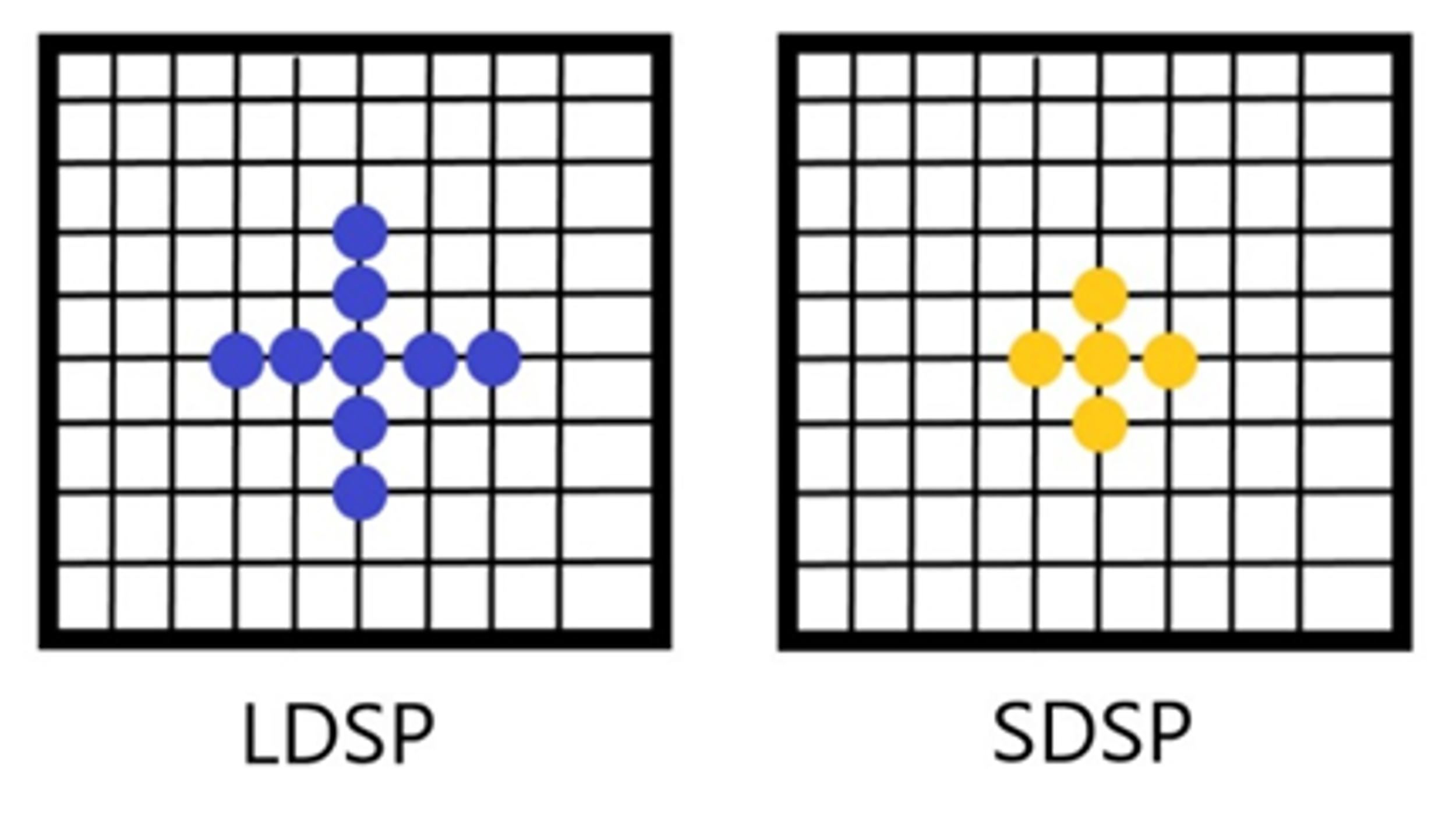
Figure 2. The template of diamond search algorithm

2.3. Spatial-temporal filtering algorithm

We utilized ME to find the best-matched block between the current frame and the reference frame, and then via motion compensation to align the current frame to the reference frame. Usually, there is temporal noise in a video sequence except spatial noise, which means the noise probably exists among the frames. When filtering the video, the larger the motion of the video block, the greater the influence of noise on the motion characteristics. The reason is that the noise in the video will lead to the larger difficulty of properly motion matching namely, the SAD will be larger. Consequently, we need to give more filtering strength for blocks with more motion intensity with a larger SAD to improve the noise reduction effect. Based on this purpose, we utilize the results of ME to calculate the residual of the best matching block and the current block. Moreover, the residual distortion will guide the proposed adaptive filtering later. Firstly, the residual of each pixel is calculated as,

\( {D_{x,y}}={{I_{C}}_{x,y}}-{{I_{R}}_{x,y}} \) , (6)

where \( {D_{x,y}} \) is the residual between the current block and the best matching block, and the average of \( {D_{x,y}} \) which named \( \bar{{\bar{D}_{x,y}}} \) is given as,

\( {\bar{D}_{x,y}}=\frac{\sum _{y=0}^{B}\sum _{x=0}^{B}{D_{x,y}}}{N} \) . (7)

Regarding equation (6) and (7), we can derive the adaptive of \( sigm{a_{r}} \) as calculated as,

\( sigm{a_{r}}=\sqrt[]{\frac{\sum _{y=0}^{B}\sum _{x=0}^{B}{( {D_{x,y}}-{\bar{D}_{x,y}})^{2}}}{N}} \) , (8)

where \( N \) is the total number of pixels of the current block. It is obvious from the equation that the larger the residual, the greater the \( sigm{a_{r}} \) , which means less filtering will be conducted by bilateral filter for blocks with less motion while vice versa. Therefore, through taking \( sigm{a_{r}} \) into (4) and combining it with (3), we can have the final adaptively block-level bilateral filtering algorithm with spatial-temporal consideration.

3. Spatial-temporal bilateral filtering by JND

JND is a psychophysical concept, which means the smallest difference between the two stimuli that a person can perceive. For spatial JND, the background luminance adaptation and texture masking are the two primary factors in the image domain [7]. The background luminance adaption is mainly influenced by luminance contrast caused by the HVS is sensitive to luminance contrast instead of absolute luminance. As for texture masking, it is well-known that the difficulty of the error finding is harder in textured areas than in smooth regions. The reason is that the increment in the texture non-uniformity in the neighborhood will lead to the decline of visibility of changes. In order to get an accurate spatial JND profile, we have to integrate the two factors due to most of the images have both varieties of masking. Therefore, Yang proposed a JND model in [7] that integrated spatial masking factors with a nonlinear additivity model for masking(NAMM) which applied to all color components and took the compound impact of luminance masking, texture masking and temporal masking into consideration. From the model, the spatial JND of each pixel can be generated as,

\( {JND_{x,y}}={{T_{l}}_{x,y}}+{{T_{t}}_{x,y}}-{C_{lt}}*min{\lbrace {{T_{l}}_{x,y}},{{T_{t}}_{x,y}}\rbrace } \) , (9)

where \( {{T_{l}}_{x,y}} \) and \( {{T_{t}}_{x,y}} \) are the visibility thresholds for the two main masking factors, background luminance adaptation and texture masking, respectively. \( {C_{lt}} \) is the overlapping coefficient. \( {{T_{l}}_{x,y}} \) can be given as,

\( {{T_{l}}_{x,y}}=\begin{cases}17(1-\sqrt[]{\frac{{\bar{I}_{x,y}}}{127}})+3 if {\bar{I}_{x,y}}≤127, \\ \frac{3({\bar{I}_{x,y}}-127)}{128}+3 otherwise,\end{cases} \) , (10)

where \( {\bar{I}_{x,y}} \) is the average background luminance of pixel position at \( (x,y) \) . Besides, the texture masking take the edge area into consideration as computed by,

\( {{T_{t}}_{x,y}}={bG_{x,y}}{E_{x,y}} \) , (11)

where \( b \) is the a control parameter for each color channel; and \( {G_{x,y}} \) is the biggest weighted average of gradients around position \( (x,y) \) . \( {E_{x,y}} \) is an edge-related weight of position \( (x,y) \) , which is calculated by edge detection followed with a Gaussian low-pass filter as,

\( {E_{x,y}}={L_{y}}*h \) , (12)

where \( {L_{y}} \) is the edge map of Y component, detected by Canny detector which is described in [11] with threshold of 0.5, and \( h \) is a 7*7 Gaussian low-pass filter with standard deviation. Moreover, \( {G_{x,y}} \) is determined as,

\( {G_{x,y}}=max⁡\lbrace \frac{\sum _{i=1}^{5}\sum _{j=1}^{5}I(x-3+i,y-3+j)∙{g_{i,j}}}{16}\rbrace \) , (13)

where \( {g_{i,j}} \) are four directional high-pass filters for texture detection which can be referred in [7].

Then after we obtain the JND of each pixel, we can combine it with equation (5), the perceptual SAD can be given as,

\( \hat{SAD}=\begin{cases}\sum _{j=0}^{B}\sum _{i=0}^{B}|{{I_{c}}_{i,j}}-{{I_{R}}_{i,j}}-{JND_{x,y}}| if|{{I_{c}}_{i,j}}-{{I_{R}}_{i,j}}| \gt {JND_{x,y}}, \\ 0 otherwise,\end{cases} \) . (14)

According to the perceptual SAD, the matching blocks which are searched by ME will be more suitable for HVS.

Finally, we can also integrate equation (9) into (6), the updated perceptual residual of each pixel \( {\hat{D}_{x,y}} \) is computed as,

\( {\hat{D}_{x,y}}=\begin{cases}|{D_{x,y}}|-{JND_{x,y}} if |{D_{x,y}}| \gt {JND_{x,y}}, \\ 0 otherwise,\end{cases} \) . (15)

Furthermore, we can combine the equation (14), (7) and (8) to obtain the perceptual \( sigm{a_{r}} \) which is calculate as,

\( \hat{sigm{a_{r}}}=\sqrt[]{\frac{\sum _{y=0}^{B}\sum _{x=0}^{B}{({\hat{D}_{x,y}}-\hat{{\bar{D}_{x,y}}})^{2}}}{N}} \) . (16)

The updated \( \hat{sigm{a_{r}}} \) will guide the result of filtering to take HVS into consideration. Based on the above process, we can implement the perception-oriented spatial-temporal video filtering algorithm which is adaptive.

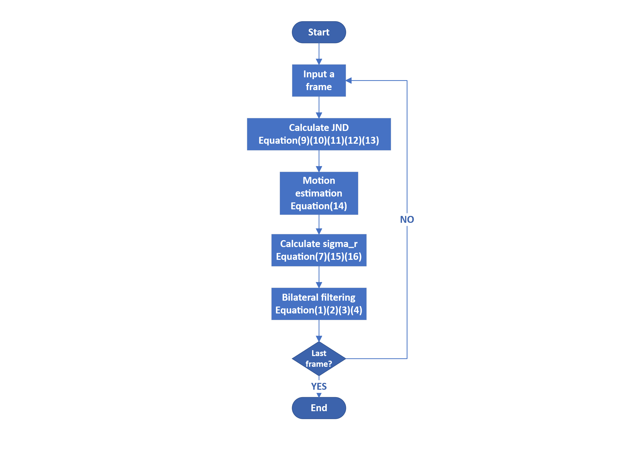
Figure 3. The flow chart of the adaptively spatial-temporal bilateral filtering based on HVS

The whole perceptual filtering process is shown in figure 3. We first calculate the JND values of the input frame. After that, we utilize the JND to perform ME on the current frame. Finally, the perceptual bilateral filtering by considering the HVS and spatial-temporal characteristics can be achieved by the perceptual filtering strength adaptively.

4. Experimental results

To verify the proposed performance of perceptually spatial-temporal bilateral filtering, we conduct several experiments including the objective and subjective quality comparison. In this experiment, we utilize the video BQMall_832x480_60 as the test sequence. The resolution of the video is 832x480 and 100 frames will be selected for evaluation. The software of our experiment is Visual Studio 2022.

Firstly, in order to evaluate comprehensive for our algorithm, the Peak Signal-to-Noise Ratio(PSNR) and Peak Signal-to-Perceptual-Noise Ratio(PSPNR)[7] metrics are both employed to give the objective and perceptual filtering quality, respectively. The PNSR is computed based on object pixel distortion \( {D_{x,y}} \) in equation (6) as calculated as,

\( PSNR=10{log_{10}}{\frac{255×255}{\frac{\sum _{x=0}^{m-1}\sum _{y=0}^{n-1} {{D_{x,y}}^{2}}}{mn}}} \) , (17)

while PSPNR is given by taking the JND into consideration as,

\( PSPNR=10{log_{10}}{\frac{255×255}{\frac{\sum _{x=0}^{m-1}\sum _{n=0}^{n-1}{{\hat{D}_{x,y}}^{2}}}{mn}}} \) . (18)

It can be seen that the \( {\hat{D}_{x,y}} \) is adjusted by JND as shown in equation (15), which means that perceptual quality can be evaluated by only taking the distortion that exceeds the JND profile into consideration.

Due to our algorithm being based on temporal filtering by ME, different ME search algorithms may affect the performance. In order to verify our method’s robustness, we separately utilize the most accurate search algorithm Full-Search (FS)[12] and a fast search algorithm DS during the temporal filtering. The results of PSNR and PSPNR of our filtering are given in table 1, respectively.

Table 1. The filtering results comparison

We can apparently see that the PSNR and PSPNR for both FS and DS are high enough, which means that the robustness is brilliant and the results are nearly not affected by the algorithm of ME namely, the accuracy of the algorithm is guaranteed. However, the runtime of DS is much less than FS. Consequently, DS is more efficient than FS in our algorithm. The average value of PSNR is relatively high with 46.13 dB, which means the filtered result is close to the initial image. Additionally, the average value of PSPNR is 54.72 much more than PSNR. Therefore, PSPNR can better reflect the perceptual filtering quality improvement of video filtering.

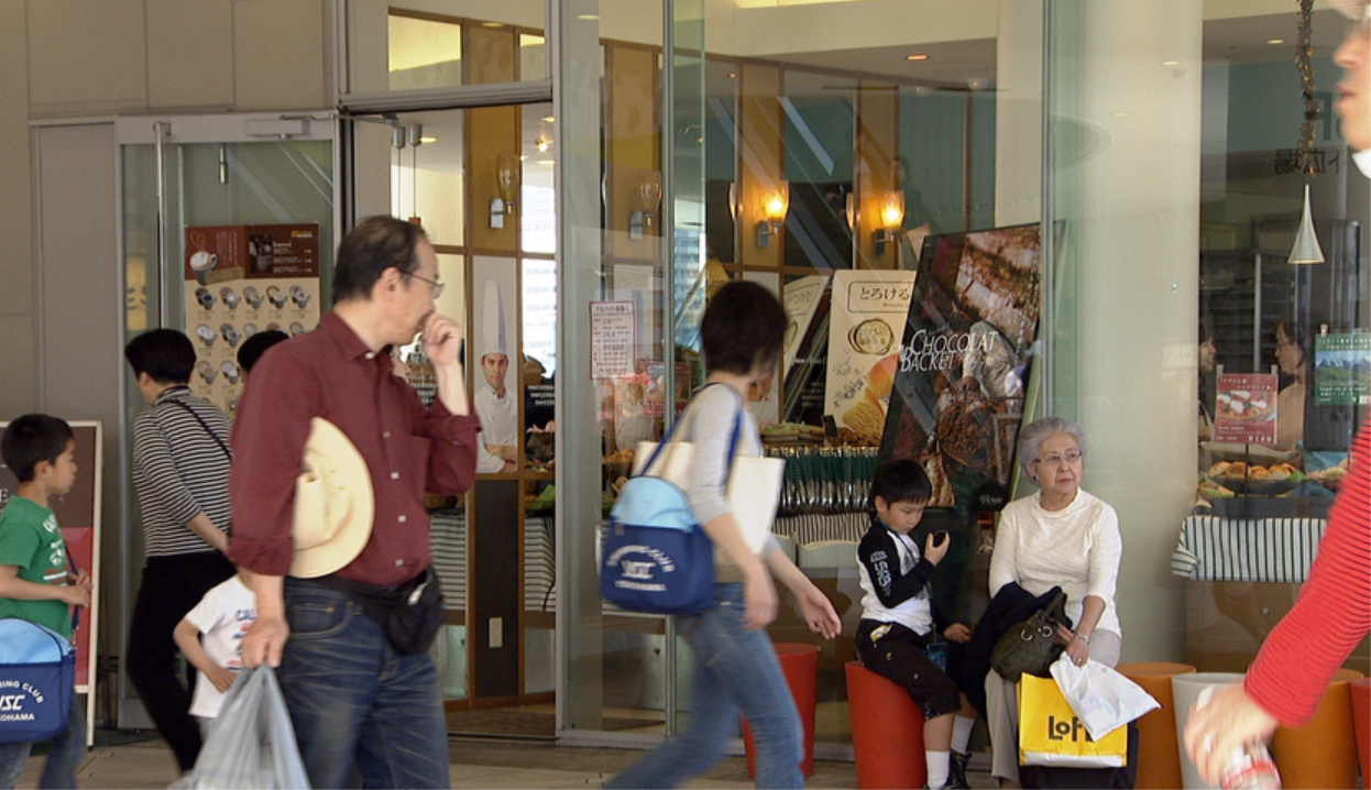
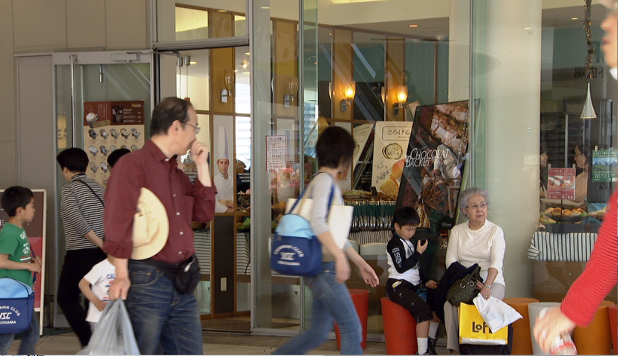
(a) The initial image of test image (b) The filtered image of test image

Finally, the subjective quality comparison between the initial and filtering images are given in figure 4. It can be seen that the visual difference between the figure 4 (a) and figure 4 (b) is negligible by human eyes. Therefore, it means that our algorithm can successfully remove unperceived noise, which is consistent with the higher PSPNR.

5. Conclusions

This paper proposes an adaptively spatial-temporal bilateral filtering algorithm that considers HVS. The algorithm includes two major methods, namely the perceptual JND based ME and spatial-temporal filtering. The JND is utilized to guide the ME process, while the bilateral filtering strength will be updated by the ME results later. The result of the experiment demonstrates that we achieve significant filtering performance both subjectively and objectively. In the future, we will continue to research better filtering algorithms, which can further improve the filtering performance.

References

[1]. Pastor D. A theoretical result for processing signals that have unknown distributions and priors in white Gaussian noise[J]. Computational statistics & data analysis, 2008, 52(6): 3167-3186.
[2]. Gavaskar R G, Chaudhury K N. Fast adaptive bilateral filtering[J]. IEEE transactions on Image Processing, 2018, 28(2): 779-790.
[3]. Papari G, Idowu N, Varslot T. Fast bilateral filtering for denoising large 3D images[J]. Ieee transactions on image processing, 2016, 26(1): 251-261.
[4]. Guo L, Au O C, Ma M, et al. A multihypothesis motion-compensated temporal filter for video denoising[C]//2006 International Conference on Image Processing. IEEE, 2006: 1417-1420.
[5]. Guo L, Au O C, Ma M, et al. Fast multi-hypothesis motion compensated filter for video denoising[J]. Journal of Signal Processing Systems, 2010, 60: 273-290.
[6]. Yahya A A, Tan J, Li L. Video Noise Reduction Method Using Adaptive Spatial‐Temporal Filtering[J]. Discrete Dynamics in Nature and Society, 2015, 2015(1): 351763.
[7]. Yang X, Ling W S, Lu Z K, et al. Just noticeable distortion model and its applications in video coding[J]. Signal processing: Image communication, 2005, 20(7): 662-680
[8]. Zhang B, Allebach J P. Adaptive bilateral filter for sharpness enhancement and noise removal[J]. IEEE transactions on Image Processing, 2008, 17(5): 664-678.
[9]. Pan Z, Lei J, Zhang Y, et al. Fast motion estimation based on content property for low-complexity H. 265/HEVC encoder[J]. IEEE Transactions on Broadcasting, 2016, 62(3): 675-684.
[10]. Priyadarshi R, Soni S K, Bhadu R, et al. Performance analysis of diamond search algorithm over full search algorithm[J]. Microsystem Technologies, 2018, 24: 2529-2537.
[11]. Canny J. A computational approach to edge detection[J]. IEEE Transactions on pattern analysis and machine intelligence, 1986 (6): 679-698.
[12]. Brunig M, Niehsen W. Fast full-search block matching[J]. IEEE Transactions on circuits and systems for video technology, 2001, 11(2): 241-247.
Cite this article
Han,Z. (2024). An adaptively perceptual video filtering algorithm. Theoretical and Natural Science,53,124-132.
Data availability
The datasets used and/or analyzed during the current study will be available from the authors upon reasonable request.
Disclaimer/Publisher's Note
The statements, opinions and data contained in all publications are solely those of the individual author(s) and contributor(s) and not of EWA Publishing and/or the editor(s). EWA Publishing and/or the editor(s) disclaim responsibility for any injury to people or property resulting from any ideas, methods, instructions or products referred to in the content.
About volume
Volume title: Proceedings of the 2nd International Conference on Applied Physics and Mathematical Modeling
© 2024 by the author(s). Licensee EWA Publishing, Oxford, UK. This article is an open access article distributed under the terms and
conditions of the Creative Commons Attribution (CC BY) license. Authors who
publish this series agree to the following terms:
1. Authors retain copyright and grant the series right of first publication with the work simultaneously licensed under a Creative Commons
Attribution License that allows others to share the work with an acknowledgment of the work's authorship and initial publication in this
series.
2. Authors are able to enter into separate, additional contractual arrangements for the non-exclusive distribution of the series's published
version of the work (e.g., post it to an institutional repository or publish it in a book), with an acknowledgment of its initial
publication in this series.
3. Authors are permitted and encouraged to post their work online (e.g., in institutional repositories or on their website) prior to and
during the submission process, as it can lead to productive exchanges, as well as earlier and greater citation of published work (See
Open access policy for details).