1. Introduction

Consider a knot, which is a one-dimensional object in the space, twisted in an arbitrary way to form a closed loop, like a shoelace, but with both ends connected. Mathematically, a knot can be understood as a continuous and injective map \( γ:{S^{1}}→{R^{3}} \) . Since \( {S^{1}} \) is compact, \( γ({S^{1}}) \) has the homeomorphism type of \( {S^{1}} \) itself. So the intrinsic topological structure of a knot \( K \) is always merely a circle, but the complexity of the way \( K \) wraps around is encoded in the map \( γ \) . The simplest example of \( γ \) is just a plain embedding, e.g. it (denoted as \( {γ_{0}} \) ) embeds \( {S^{1}} \) as

\( \lbrace (x,y,z)∈{R^{3}}|{x^{2}}+{y^{2}}=1,z=0\rbrace \) (1)

Such a knot is completely without entanglement. When \( γ \) as a map becomes complicated, the knot \( K \) might be entangled "in an essential way". The following formal definition of the isotopy relation between knots captures the intuitive process of deforming a knot.

Definition 1.1. An isotopy from a knot \( ({K_{1}};{γ_{1}}) \) to another knot \( ({K_{2}};{γ_{2}}) \) is a homotopy \( f:{S^{1}}×[0,1]→{R^{3}} \) from \( {γ_{1}} \) to \( {γ_{2}} \) (meaning a continuous map with \( f(-,0)={γ_{1}} \) , \( f(-,1)={γ_{2}} \) ), such that \( ∀t∈[0,1] \) , \( f(-,t) \) is always a knot, in the sense mentioned above. If such an \( f \) exists, we say that \( {K_{1}} \) and \( {K_{2}} \) are isotopic, or equivalent.

Definition 1.2. Any knot equivalent to \( {γ_{0}} \) defined by 1.1 is said to be an unknot, or can be unknotted.

Sometimes in practice, additional structure needs to be put on a knot to study it, namely the smooth structure. So we view \( γ \) as a smooth map between the smooth manifolds \( {S^{1}} \) and \( {R^{3}} \) , hence we can speak of the tangent map \( {γ^{ \prime }} \) . Since the shape of the knot is determined only by the image of \( γ \) , we can choose any reparameterization. We can always choose one that satisfies the uniformization convention: the tangent vectors are unit vectors everywhere (called the arc length reparameterization). To summarize, we now revise our definition of knots as follows.

Definition 1.3. A knot \( K \) is a smooth embedding \( γ \) from the quotient manifold \( R/L≅{S^{1}} \) to \( {R^{3}} \) (i.e. a smooth map \( γ=({γ_{1}},{γ_{2}},{γ_{3}}):R→{R^{3}} \) with \( γ(t)=γ(t+L) \) ), such that \( |{γ^{ \prime }}(t)|=1 \) , \( ∀t∈R \) . The number \( L \) is the length of \( K \) .

Definition 1.4. The local curvature of \( K \) is a function defined as

\( κ(t)=|{γ^{ \prime \prime }}(t)|, ∀t∈R. \) (2)

The total curvature of \( K \) is a number that is the integration of local curvatures:

\( {T_{K}}:=\int _{0}^{L}κ(t)dt. \) (3)

The local curvature reflects how curved the knot is locally at a point \( γ(t) \) : \( κ(t) \) is large when bending very sharply, small when barely bending (and 0 when it is locally just a flat line). Imagine the knot as the trajectory of a uniform motion, then the curvature represents the magnitude of acceleration. The larger it is, the faster the point deviates. If we integrate all the local curvatures together, we obtain a quantity that measures the overall twistedness of the knot. The following result (to be proved) is a quantitative way of saying that for a knot to be linked head-to-tail, it has to be "sufficiently curved".

Theorem 1.5. \( {T_{K}}≥2π \) , for any knot \( K \) .

The next result, originally proved by Fáry [1] and Milnor [2] and reviewed in [3], is a central problem that we are going to address in this article. Intuitively, it says that if a knot is not "curved enough", then it can be unknotted.

Theorem 1.6. If \( {T_{K}} \lt 4π \) , then \( K \) is an unknot.

Example. Take the trefoil knot for example. It can be wrapped around a torus as below:

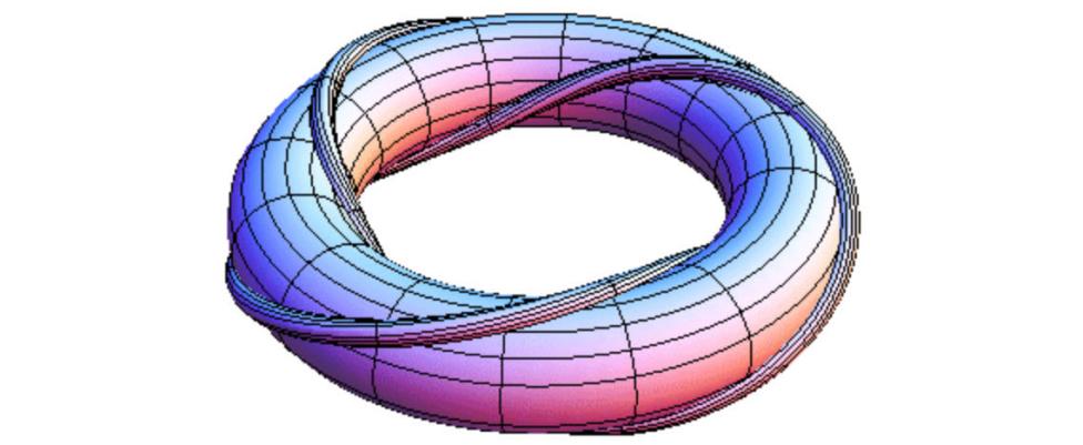
Figure 1: Picture taken from https://mathoverflow.net/questions/91444.

It is essentially entangled (can not be unknotted, see [4]). The torus surface can be defined by the equation in terms of \( (rcosθ,rsinθ,z) \) :

\( {(r-2)^{2}}+{z^{2}}=1. \) (4)

Observing how the trefoil knot is wrapped on that surface, we can give it a parameterization:

\( γ(t)=((2+cos3t)cos2t,(2+cos3t)sin2t,sin3t), t∈[0,2π]. \) (5)

It is not an arc length parameterization. Nevertheless there is still a formula computing the curvature ([5] theorem 7.15):

\( κ=\frac{|{γ^{ \prime }}×{γ^{ \prime \prime }}|}{{|{γ^{ \prime }}|^{3}}} \) (6)

where \( × \) is the cross product. Plugging in the formula of \( γ \) , a software computation reveals that

\( T=\int _{0}^{2π}κ(t)dt \gt 4π. \) (7)

This does not violate the Fáry-Milnor theorem. Note that the theorem states that \( {T_{K}} \lt 4π \) implies unknot, but does not say anything when \( {T_{K}}≥4π \) . In fact, no matter how we deform the trefoil knot, the total curvature can not be less than \( 4π \) .

Remark 1.7. We emphasize that whether a knot is an unknot or not is a topological statement. It is a well-defined property that does not depend on which specific smooth structure / parameterization is given to the knot. So in the Fáry-Milnor theorem, we are studying this topological property of a knot through the lens of smooth data on it, i.e. the curvatures.

The method that we are going to employ to prove the theorem, besides basic vector calculus, is the Morse theory, which does not show up explicitly in the original papers of Fáry-Milnor. It is a rich and beautiful theory in its own right. We will give a quick review of its basics in section 2. In section 3 we illustrate this theory with a simple and non trivial example \( {RP^{n}} \) . We find this example very much exhibits the essence of Morse theory. After these preparatory works, we present in detail a proof of the Fáry-Milnor theorem in section 4. In the last section we study the discrete Morse theory. The key is to elucidate how the concepts in classical Morse theory are parallelly borrowed in the setting of discrete world. Then as an application, we discuss how the discrete Morse theory is related to the computation of simplicial homology.

2. Review of Morse theory

We state the basic results in classical Morse theory. The standard reference is [6] or [7]. First we need some definitions. Throughout, \( M \) is a compact smooth manifold of dimension \( n \) , and \( f∈{C^{∞}}(M) \) is a smooth function on it.

Definition 2.1 For \( x∈M \) , let \( {∇_{x}}f \) denote the induced linear map on the tangent spaces

\( {∇_{x}}f:{T_{x}}M→{T_{f(x)}}R=R. \) (8)

In a local coordinate, we can represent the map as a \( 1×n \) matrix:

\( {∇_{x}}f=(\frac{∂f}{∂{x_{1}}}(x),⋯,\frac{∂f}{∂{x_{n}}}(x)). \) (9)

This is called the gradient of \( f \) at \( x \) .

Fix an embedding into Euclidean space of \( M \) (which is always possible by Whitney’s theorem, see [8] theorem 6.15). Often by abus of notation, we understand \( {∇_{x}}f \) as an element in \( {T_{x}}M \) (i.e. a tangent vector):

\( {∇_{x}}f=\sum _{i=1}^{n}\frac{∂f}{∂{x_{i}}}(x)\cdot \frac{∂}{∂{x_{i}}} \) (10)

where \( \lbrace \frac{∂}{∂{x_{i}}}\rbrace \) is chosen to be an orthonormal basis of \( {T_{x}}M \) . This is well-defined (does not depend on the choice of the basis \( \lbrace \frac{∂}{∂{x_{i}}}\rbrace \) ), and represents the vector of steepest ascent of \( f \) at \( x \) .

Definition 2.2 A critical point of \( f \) is a point \( p∈M \) such that \( {∇_{p}}f=0 \) .

Concretely, this means that \( f \) has 0 rate of change along any direction at \( p \) .

Morse lemma. At a critical point \( p \) , there is a local coordinate chart \( ({x_{i}}) \) (called a standard coordinate chart) centered at \( p \) (meaning \( p=(0,⋯,0) \) ) in which \( f \) can be locally expressed as

\( f(x)=-x_{1}^{2}-⋯-x_{λ}^{2}+x_{λ+1}^{2}+⋯+x_{μ}^{2}. \) (11)

Moreover, the numbers \( 0≤λ≤μ≤n \) are uniquely determined by \( f \) and the point \( p \) . We say that \( λ \) is the index of \( p \) .

As a consequence, critical points are isolated hence finitely many (since \( M \) is compact).

Definition 2.3. A critical point is said to be non degenerate if \( μ=n \) , and \( f \) is said to be a Morse function if all critical points of \( f \) are non degenerate.

As a smooth vector field, \( ∇f \) determines a flow called the gradient flow \( X(t) \) (a smooth curve on \( M \) ) in the sense that

\( {X^{ \prime }}(t)={∇_{X(t)}}f. \) (12)

Such a curve / flow always exists locally due to the theorem of existence and uniqueness of solutions of ordinary differential equations (known as the Picard-Lindelöf theorem, [9] theorem 2.2). If we consider the gradient flow determined by \( -\frac{∇f}{{|∇f|^{2}}} \) (i.e. the same flow curve but with a reparameterization), then ([6] theorem 3.1) we have a uniform descent and it turns out that:

The 1st fundamental theorem of Morse theory. Denote \( {M_{c}}:={f^{-1}}(-∞,c] \) , \( c∈R \) . If \( a \lt b \) and \( {f^{-1}}[a,b] \) contains no critical point, then we have a diffeomorphism \( {M_{a}}≅{M_{b}} \) .

In the case of the presence of critical points, we have another result ( theorem 3.2):

The 2nd fundamental theorem of Morse theory. If \( {f^{-1}}[a,b] \) contains one critical point \( p \) and it is non degenerate of index \( λ \) , then \( M(b) \) deformation retracts onto \( M(a) \) with a \( λ \) -dimensional cell \( {e^{λ}} \) attached (at the boundary), so that we have a homotopy equivalence \( M(b)≃M(a)∪{e^{λ}} \) .

Put together, we conclude that if \( f \) is a Morse function with \( k \) critical points of indices \( {λ_{1}}≤⋯≤{λ_{k}} \) respectively, then \( M \) has the homotopy type \( {e^{{λ_{1}}}}∪⋯∪{e^{{λ_{k}}}} \) of a cell complex (see the appendix of [10]) of exactly \( k \) cells, one for each critical point of \( f \) .

Remark 2.4. A subtle issue arises when two critical points happen to have the same value. But it turns out that one can always perturb \( f \) slightly so that the values are distinct (while preserving the indices), then the conclusion follows from the two fundamental theorems of Morse theory.

3. Morse theory on the real projective space \( {RP^{n}} \)

In this section we work out explicitly the Morse theory when applied to \( {RP^{n}} \) , the real projective space. Though there is no logical dependence for the subsequent sections, we found this explicit example very helpful during the author’s studying process of Morse theory.

3.1. \( {RP^{n}} \) as a manifold

The space \( {RP^{n}} \) is defined as consisting of all lines in \( {R^{n+1}} \) passing through the origin. As a quotient space,

\( {RP^{n}}=\lbrace ({x_{0}},{x_{1}},⋯,{x_{n}})∈{R^{n+1}}-\lbrace 0\rbrace |({x_{0}},⋯,{x_{n}})∼(λ{x_{0}},⋯,λ{x_{n}}), λ∈R-\lbrace 0\rbrace \rbrace \) (13)

or equivalently

\( {RP^{n}}={S^{n}}/\lbrace ±1\rbrace =\lbrace ({x_{0}},⋯,{x_{n}})∈{R^{n+1}}|\sum _{i=0}^{n}x_{i}^{2}=1\rbrace /({x_{0}},⋯,{x_{n}})∼(-{x_{0}},⋯,-{x_{n}}). \) (14)

Proposition 3.1. \( {RP^{n}} \) is a compact smooth manifold of dimension \( n \) .

Proof: Since \( {S^{n}} \) is compact, \( {RP^{n}} \) is compact as its quotient space. To show the smoothness, we construct a coordinate atlas as follows. In 3.1 we denote the equivalence class of \( ({x_{0}},⋯,{x_{n}}) \) as \( [{x_{0}},⋯,{x_{n}}] \) (the homogeneous coordinate). Notice that \( {RP^{n}} \) is covered by \( n+1 \) open subsets

\( {U_{i}}:=\lbrace [{x_{0}},{x_{1}},⋯,{x_{n}}]|{x_{i}}≠0\rbrace , i=0,1,⋯,n. \) (15)

On each \( {U_{i}} \) , we have a well-defined continuous map \( {φ_{i}}:{U_{i}}→{R^{n}} \) as

\( {φ_{i}}([{x_{0}},{x_{1}},⋯,{x_{n}}])=(\frac{{x_{0}}}{{x_{i}}},⋯,\frac{{x_{i-1}}}{{x_{i}}},\frac{{x_{i+1}}}{{x_{i}}},⋯,\frac{{x_{n}}}{{x_{i}}}) \) (16)

with a continuous inverse

\( φ_{i}^{-1}({a_{1}},⋯,{a_{n}})=[{a_{1}},⋯,{a_{i}},1,{a_{i+1}},⋯,{a_{n}}]. \) (17)

It follows that \( {φ_{i}} \) is a homeomorphism, hence defines a coordinate chart of \( {U_{i}} \) . For \( i \lt j \) , on \( {U_{i}}∩{U_{j}}=\lbrace [{x_{0}},{x_{1}},⋯,{x_{n}}]|{x_{i}},{x_{j}}≠0\rbrace \) , the coordinate transformation

\( {φ_{j}}∘φ_{i}^{-1}({a_{1}},⋯,{a_{n}})=(\frac{{a_{1}}}{{a_{j}}},⋯,\frac{{a_{i}}}{{a_{j}}},\frac{1}{{a_{j}}},⋯,\frac{{a_{j-1}}}{{a_{j}}},\frac{{a_{j+1}}}{{a_{j}}},⋯,\frac{{a_{n}}}{{a_{j}}}) \) (18)

is a smooth map. We conclude that \( \lbrace {U_{i}};{φ_{i}}{\rbrace _{i=0,1,⋯,n}} \) is a smooth atlas, and \( {RP^{n}} \) is a smooth manifold of dimension \( n \) . \( ▫ \)

3.2. A Morse function on \( {RP^{n}} \)

In this subsection we construct a function on \( {RP^{n}} \) and show that it is a Morse function.

The construction of the function. Take an arbitrary sequence of numbers \( {c_{0}} \lt {c_{1}} \lt ⋯ \lt {c_{n}} \) . Consider the smooth function

\( \widetilde{f}({x_{0}},{x_{1}},⋯,{x_{n}})=\sum _{i=0}^{n} {c_{i}}x_{i}^{2} \) (19)

on \( {R^{n+1}} \) . It restricts to a smooth function \( \widetilde{f}{|_{{S^{n}}}} \) on the unit sphere \( {S^{n}} \) , which then descends to a function \( f \) on \( {RP^{n}} \) via the identification [sn]. That is,

\( \widetilde{f}{|_{{S^{n}}}}={f^{∘}}q \) (20)

where \( q \) denotes the quotient map \( {S^{n}}→{S^{n}}/\lbrace ±1\rbrace ={RP^{n}} \) .

Proposition 3.2. \( f \) is a well-defined smooth function.

Proof: It is well-defined since

\( \widetilde{f}({x_{0}},{x_{1}},⋯,{x_{n}})=\widetilde{f}(-{x_{0}},-{x_{1}},⋯,-{x_{n}}). \) (21)

As a polynomial, it is clearly smooth. \( ▫ \)

We can easily compute the gradient of \( \widetilde{f} \) :

\( {∇_{x}}\widetilde{f}=(\frac{∂\widetilde{f}}{∂{x_{0}}}(x),⋯,\frac{∂\widetilde{f}}{∂{x_{n}}}(x))=2({c_{0}}{x_{0}},⋯,{c_{n}}{x_{n}}),x=({x_{0}},⋯,{x_{n}})∈{R^{n+1}}. \) (22)

Since the tangent space of \( {S^{n}} \) is included into that of \( {R^{n+1}} \) as

\( {T_{x}}{S^{n}}=\lbrace ({y_{0}},⋯,{y_{n}})|({y_{0}},⋯,{y_{n}})⊥({x_{0}},⋯,{x_{n}})\rbrace ↪{T_{x}}{R^{n+1}}={R^{n+1}} \) (23)

the tangent map induced by \( \widetilde{f}{|_{{S^{n}}}} \) is

\( {∇_{x}}\widetilde{f}{∣_{{S^{n}}}}\cdot {T_{x}}{S^{n}}→R,({y_{0}},⋯,{y_{n}})↦\sum _{i=0}^{n} 2{c_{i}}{x_{i}}{y_{i}}=2({c_{0}}{x_{0}}⋯,{c_{n}}{x_{n}})\cdot ({y_{0}}⋯,{y_{n}}). \) (24)

By the chain rule and 3.8 we have

\( {∇_{x}}\widetilde{f}{|_{{S^{n}}}}={∇_{x}}{f^{∘}}{q_{*,x}} \) (25)

where the tangent map \( {q_{*,x}}:{T_{x}}{S^{n}}→{T_{x}}{RP^{n}} \) is an isomorphism. We deduce that

\( {∇_{x}}f=0⇔{∇_{x}}\widetilde{f}{∣_{{S^{n}}}}=0⇔({c_{0}}{x_{0}},⋯,{c_{n}}{x_{n}})∈({T_{x}}{S^{n}}{)^{⊥}}=R\cdot ({x_{0}}⋯,{x_{n}}). \) (26)

But the \( {c_{i}} \) ’s are distinct to each other, we have \( ({c_{0}}{x_{0}},⋯,{c_{n}}{x_{n}}) \) is colinear with \( ({x_{0}},⋯,{x_{n}}) ⇔ \) all but one \( {x_{i}} \) are zero. In conclusion, we have shown that

Proposition 3.3. The critical points of \( f \) are

\( {p_{0}}:=[1,0,⋯,0], {p_{1}}:=[0,1,0,⋯,0], ⋯, {p_{n}}:=[0,⋯,0,1] \) (27)

To show that \( f \) is a Morse function, it remains to show that each \( {p_{i}} \) is non degenerate. In fact

Proposition 3.4. \( {p_{i}} \) is non degenerate with index \( i \) .

Proof: Consider the open subset \( {V_{i}}⊂{S^{n}} \) defined by

\( {V_{i}}=\lbrace ({x_{0}},⋯,{x_{n}})∈{S^{n}}|{x_{i}} \gt 0\rbrace . \) (28)

Then the projection map

\( {ψ_{i}}:{V_{i}}→{R^{n}}, ({x_{0}},⋯,{x_{n}})↦({x_{0}},⋯,{x_{i-1}},{x_{i+1}},⋯,{x_{n}}) \) (29)

is a homeomorphism onto the image of \( {ψ_{i}} \) , thus makes \( {V_{i}} \) into a local coordinate chart centered at \( {p_{i}} \) . On this chart we can write \( f \) as

\( f{|_{{V_{i}}}}∘ψ_{i}^{-1}:({x_{0}},⋯,{x_{i-1}},{x_{i+1}},⋯,{x_{n}})↦\sum _{i=0}^{n}{c_{i}}x_{i}^{2}={c_{i}}+\sum _{j≠i}^{​}({c_{j}}-{c_{i}})x_{j}^{2} \) (30)

where we have used the relation

\( {x_{i}}=\sqrt[]{1-\sum _{j≠i}^{​}x_{j}^{2}}. \) (31)

Since \( {c_{j}}-{c_{i}} \lt 0 \) for \( j \lt i \) , and \( {c_{j}}-{c_{i}} \gt 0 \) for \( j \gt i \) , locally at \( {p_{i}} \) , \( f \) has exactly \( i \) negative directions and \( n-i \) positive directions. A dilation transformation

\( ({x_{0}},⋯,{x_{i-1}},{x_{i+1}},⋯,{x_{n}})↦(\frac{{x_{0}}}{\sqrt[]{{c_{i}}-{c_{0}}}},⋯,\frac{{x_{i-1}}}{\sqrt[]{{c_{i}}-{c_{i-1}}}},\frac{{x_{i+1}}}{\sqrt[]{{c_{i+1}}-{c_{i}}}},⋯,\frac{{x_{n}}}{\sqrt[]{{c_{n}}-{c_{i}}}}) \) (32)

takes \( f \) into a standard form as in the Morse lemma. We thus conclude that \( {p_{i}} \) is non degenerate with index \( i \) . \( ▫ \)

3.3. Applying the Morse theory

Now we can inspect what the Morse theory states for this particular Morse function \( f \) on \( {RP^{n}} \) . By applying the two fundamental theorems of Morse theory we arrive at:

Proposition 3.5. \( {RP^{n}} \) has the homotopy type \( {e^{0}}∪{e^{1}}∪⋯∪{e^{n}} \) .

In fact, we know that this is exactly the cell decomposition of \( {RP^{n}} \) . Consider the equator \( {S^{n-1}} \) in \( {S^{n}} \) , then

\( {RP^{n-1}}={S^{n-1}}/\lbrace ±1\rbrace ⊂{RP^{n}}={S^{n}}/\lbrace ±1\rbrace \) (33)

and \( {RP^{n}}-{RP^{n-1}} \) can be identified with a hemisphere that is, an \( n \) -dimensional cell. The upshot is that the Morse function \( f \) , which is a smooth datum, indeed provides us with some useful topological information about \( {RP^{n}} \) .

4. Proving the Fáry-Milnor theorem

We are now ready to prove theorem 1.5 and 1.6. To use Morse theory, we will employ height functions to supply Morse functions on \( K \) . Precisely, for any \( v∈{S^{2}} \) the unit sphere of \( {R^{3}} \) , consider the height function \( {h_{v}} \) on \( K \) along \( v \)

\( {h_{v}}(x):=⟨x,v⟩ \) (34)

where \( ⟨-,-⟩ \) is the inner product on \( {R^{3}} \) . Denote by \( μ(v) \) the number of critical points of \( {h_{v}} \) . The key in our proof is to show that the total curvature naturally emerges in the averaging process of the numbers \( μ(v) \) :

\( \frac{{T_{K}}}{π}=\frac{1}{4π}\int _{{S^{2}}}^{​}μ(v)dv. \) (35)

Then we will subsequently show that

Proposition 4.1. If \( {T_{K}} \lt 4π \) , there exists an element \( v∈{S^{2}} \) such that \( μ(v)=2 \) .

Proposition 4.2. If \( {h_{v}} \) has exactly two critical points, then \( K \) can be unknotted.

We start with deriving the equation 35.

4.1. The Morse functions \( {h_{v}} \)

First of all, not all height functions \( {h_{v}} \) are Morse functions. We will characterize the condition on \( v \) such that \( {h_{v}} \) is not a Morse function. On such points \( v∈{S^{2}} \) , \( μ(v) \) is ill-defined. However, we will see that such points form a measure zero subset of \( {S^{2}} \) , hence do not affect the integral in35.

We first characterize the condition of \( γ(s)∈K \) being a critical point of \( {h_{v}} \) . In the local coordinate \( (s) \) of \( K \) , since \( {h_{v}}(s)=⟨γ(s),v⟩ \) , we have

\( ∇{h_{v}}=h_{v}^{ \prime }(s)=⟨{γ^{ \prime }}(s),v⟩. \) (36)

The gradient at \( γ(s) \) vanishes if and only if \( v⊥{γ^{ \prime }}(s) \) . This motivates the following definition.

Definition 4.3. Let \( S(K) \) be a surface defined as

\( S(K):=\lbrace (γ(s),v)∈K×{S^{2}}|v⊥{γ^{ \prime }}(s),s∈R\rbrace . \) (37)

Proposition 4.4. \( S(K) \) is a smooth manifold of dimension 2.

Proof: Recall that \( {γ^{ \prime }}(s) \) is a unit vector. Consider the open submanifold of \( K×{R^{3}} \) defined as

\( \widetilde{S}(K):=\lbrace (γ(s),ν)∈K×{R^{3}}|visnotcolinearwith{γ^{ \prime }}(s)\rbrace . \) (38)

Let \( f:\widetilde{S}(K)→{R^{2}} \) be a smooth map defined as

\( f:(γ(s),v)↦(v\cdot {γ^{ \prime }}(s),v\cdot v) \) (39)

where denotes the inner product. Since its Jacobian matrix

\( J(f)=(\begin{matrix}v\cdot {γ^{ \prime \prime }}(s) & {γ^{ \prime }}(s) \\ 0 & 2v \\ \end{matrix}) \)

is of full rank everywhere ( \( 2v \) is not colinear with \( {γ^{ \prime }}(s) \) ), by the constant rank theorem ( theorem 5.12), \( S(K)={f^{-1}}(0,1) \) is a regular submanifold of \( \widetilde{S}(K) \) of codimension 2. Thus \( S(K) \) is a smooth manifold of dimension 2. \( ▫ \)

Remark 4.5. For a given \( γ(s) \) on the knot, the points \( v \) such that \( v⊥{γ^{ \prime }}(s) \) form a great circle of \( {S^{2}} \) . In formal language, we say that \( S(K) \) is the normal circle bundle on \( K \) . Intuitively, we can think of \( S(K) \) as the surface of a rope representing \( K \) with thickness. This is justified by the following result.

Proposition 4.6. \( S(K) \) can be embedded into \( {R^{3}} \) via

\( S(K)↪{R^{3}}, (γ(s),v)↦γ(s)+ϵv \) (40)

for a sufficient small constant \( ϵ \gt 0 \) .

Proof: This directly follows from the tubular neighborhood theorem ( theorem 6.24). Alternatively, we can sketch a proof without invoking the theorem. By the compactness of \( K \) , let \( M \) be the maximum of the local curvatures \( κ(s)=|{γ^{ \prime \prime }}(s)| \) . We can choose \( ϵ∈(0,\frac{1}{2M}) \) such that every ball of radius \( ϵ \) intersects \( K \) at a connected interval of length \( \lt \frac{1}{M} \) (again by the compactness). We show that \( ∄γ({s_{1}})+ϵ{v_{1}}=γ({s_{2}})+ϵ{v_{2}} \) for \( {s_{1}} \lt {s_{2}} \) , so that \( ϵ \) satisfies the requirement. If such \( {s_{1}} \) and \( {s_{2}} \) exist, then \( {s_{2}}-{s_{1}} \lt \frac{1}{M} \) . Thus

\( |{γ^{ \prime }}(s)-{γ^{ \prime }}({s_{1}})|≤(s-{s_{1}})M \lt 1, ∀s∈[{s_{1}},{s_{2}}]. \) (41)

That is, \( {γ^{ \prime }}(s),{γ^{ \prime }}({s_{1}})∈{S^{2}} \) have central angle \( \lt \frac{π}{3} \) . This implies that the distance from \( γ({s_{2}}) \) to the normal plane \( {P_{1}} \) at \( γ({s_{1}}) \) is at least \( ({s_{2}}-{s_{1}})cos\frac{π}{3}=\frac{{s_{2}}-{s_{1}}}{2} \) . Moreover, if \( α \) is the dihedral angle between the normal plane \( {P_{2}} \) at \( γ({s_{2}}) \) and \( {P_{1}} \) , then \( sinα \lt ({s_{2}}-{s_{1}})M \) . We conclude that the distance from \( γ({s_{2}}) \) to \( {P_{1}}∩{P_{2}} \) is at least \( \frac{{s_{2}}-{s_{1}}}{2sinα} \gt \frac{1}{2M} \gt ϵ \) , a contradiction. \( ▫ \)

From now on, we will make no distinction between \( S(K) \) and the embedded manifold, and \( ϵ \) will be suppressed. The embedding enables us to speak of \( {T_{x}}S(K) \) as an inner product space. Along the great circle, we have a tangent vector \( \frac{∂}{∂θ}∈{T_{x}}S(K) \) . Perpendicular to it, we have \( \frac{∂}{∂s} \) ("along the knot") so that \( \lbrace \frac{∂}{∂s},\frac{∂}{∂θ}\rbrace \) forms an orthonormal basis of \( {T_{x}}S(K) \) .

Remark 4.7. To motivate the notation \( \frac{∂}{∂s} \) , notice that the tangent plane \( {T_{x}}S(K) \) is parallel to \( {γ^{ \prime }}(s) \) (where \( x=(γ(s),v) \) ), hence \( \frac{∂}{∂s} \) can be viewed as the same vector as \( {γ^{ \prime }}(s) \) . To see this, consider an arbitrary curve \( γ(s)+v(s) \) on \( S(K) \) . We have

\( ⟨{γ^{ \prime }}(s)+{v^{ \prime }}(s),v(s)⟩=⟨{γ^{ \prime }}(s),v(s)⟩+⟨{v^{ \prime }}(s),v(s)⟩=0 \) (42)

where \( ⟨{γ^{ \prime }}(s),v(s)⟩=0 \) follows from the definition of \( S(K) \) , \( ⟨{v^{ \prime }}(s),v(s)⟩=0 \) follows from \( |v(s)|≡1 \) . So all tangent vectors are perpendicular to \( v(s) \) , hence the tangent plane is parallel to \( {γ^{ \prime }}(s) \) .

Consider the natural projection

\( p:S(K)→{S^{2}}, (γ(s),v)↦v. \) (42)

Proposition 4.8. If \( {h_{v}} \) is not a Morse function, then \( v \) is a critical value of \( p \) .

Proof: If so, there is a degenerate critical point \( γ({s_{0}}) \) . Recall that \( γ({s_{0}}) \) being a critical point means \( x:=(γ({s_{0}}),v)∈S(K) \) . We show that \( {p_{*}}:{T_{x}}S(K)→{T_{v}}{S^{2}} \) is not surjective, hence \( v \) is a critical value. The \( γ({s_{0}}) \) being degenerate means the Hessian matrix of \( {h_{v}} \) at it is singular ([6], section 1.2). In our case, the Hessian matrix is just the \( 1×1 \) matrix \( h_{v}^{ \prime \prime }({s_{0}})={γ^{ \prime \prime }}({s_{0}})\cdot v \) so it is zero. For any curve \( (γ(s),v(s)) \) passing through \( x \) on \( S(K) \) , since \( {γ^{ \prime }}(s)\cdot v(s)≡0 \) , taking derivative at \( {s_{0}} \) yields

\( 0={γ^{ \prime \prime }}({s_{0}})\cdot v+{γ^{ \prime }}({s_{0}})\cdot {v^{ \prime }}({s_{0}})={γ^{ \prime }}({s_{0}})\cdot {v^{ \prime }}({s_{0}}). \) (43)

That is, \( {v^{ \prime }}({s_{0}})∈{γ^{ \prime }}{({s_{0}})^{⊥}} \) which is a 1-dimensional subspace of \( {T_{v}}{S^{2}} \) . Hence \( {p_{*}} \) is not surjective (in fact \( {p_{*}} \) is of rank 1 with image generated by \( {p_{*}}(\frac{∂}{∂θ}) \) ). \( ▫ \)

Corollary 4.9. The points \( v∈{S^{2}} \) such that \( {h_{v}} \) is not Morse form a measure zero subset.

Proof: This follows from Sard’s theorem ([8] theorem 6.10). \( ▫ \)

4.2. Evaluating the integral

We just proved that the integral in 35 is well-defined, now we evaluate it. Recall that \( μ(v) \) as the number of critical points of \( {h_{v}} \) can be expressed as

\( μ(v)=|\lbrace γ(s)∈K|(γ(s),v)∈S(K)\rbrace |. \) (44)

Hence \( μ(v) \) is exactly the cardinality of the preimage \( {p^{-1}}(v) \) .

Proposition 4.10. At each point \( x∈S(K) \) we define \( {x_{s}}:={p_{*}}(\frac{∂}{∂s}) \) , \( {x_{θ}}:={p_{*}}(\frac{∂}{∂θ}) \) , and a matrix

\( G(x):=(\begin{matrix}⟨{x_{s}},{x_{s}}⟩ & ⟨{x_{s}},{x_{θ}}⟩ \\ ⟨{x_{θ}},{x_{s}}⟩ & ⟨{x_{θ}},{x_{θ}}⟩ \\ \end{matrix}). \) (45)

Then we have

\( \int _{S(K)}^{​}\sqrt[]{det(G)}dsdθ=\int _{{S^{2}}}^{​}μ(v)dv. \) (46)

Proof: This is the coarea formula ([11] theorem 3.11). However, we can sketch an informal heuristic argument. The matrix \( G(x) \) is so defined that \( \sqrt[]{det(G(x))} \) is the local ratio induced by \( p \) at \( x \) of infinitesimal areas. Explicitly, we can compute the determinant as

\( det(G(x))={|{x_{s}}|^{2}}{|{x_{θ}}|^{2}}-{(|{x_{s}}||{x_{θ}}|cosα)^{2}}={|{x_{s}}|^{2}}{|{x_{θ}}|^{2}}si{n^{2}}α \) (47)

where \( α \) is the angle between \( {x_{s}} \) and \( {x_{θ}} \) in \( {T_{p(x)}}{S^{2}} \) . This is exactly the squared area of the infinitesimal parallelogram spanned by \( {x_{s}},{x_{θ}} \) . Recall that \( \lbrace \frac{∂}{∂s},\frac{∂}{∂θ}\rbrace \) is an orthonormal basis, we conclude that infinitesimally \( p \) scales up the area element \( dsdθ \) of \( S(K) \) into \( {S^{2}} \) by the scalar \( \sqrt[]{det(G)} \) . Integrating \( \sqrt[]{det(G)}dsdθ \) on \( S(K) \) is to integrate a weighted area element on \( {S^{2}} \) , where \( dv \) is weighted \( μ(v)=|{p^{-1}}(v)| \) times since \( v \) is covered such many times under \( p \) . \( ▫ \)

To evaluate \( \int _{S(K)}^{​}\sqrt[]{det(G)}dsdθ \) , we first integrate along \( θ \) (i.e. along the great circles):

Proposition 4.11. For each \( s \) ,

\( \int _{0}^{2π}\sqrt[]{det(G)}dθ=4κ(s). \) (48)

This section will culminate at this central result. We will give two proofs, one is computational, and one is conceptual and informal. Note that equation 35 will be derived from this:

\( \frac{{T_{K}}}{π}=\frac{1}{π}\int _{0}^{L}κ(s)ds=\frac{1}{4π}\int _{S(K)}^{​}\sqrt[]{det(G)}dsdθ=\frac{1}{4π}\int _{{S^{2}}}^{​}μ(v)dv. \) (49)

Proof: (Computational.) To compute, we choose a local orthonormal moving frame \( \lbrace {γ^{ \prime }}(s),{e_{1}}(s),{e_{2}}(s)\rbrace \) along \( K \) , where \( {e_{1}}(s) \) is a flow curve on \( S(K) \) generated by \( \frac{∂}{∂s} \) , and \( {e_{2}}(s)={γ^{ \prime }}(s)×{e_{1}}(s) \) . We can think of \( {e_{1}}(s) \) / \( {e_{2}}(s) \) as marking the curve \( θ=0 \) / \( θ=\frac{π}{2} \) . We can thus express the map \( p \) in terms of local coordinate

\( p(s,θ)=cosθ{e_{1}}(s)+sinθ{e_{2}}(s). \) (50)

It then follows that

\( {x_{s}}=cosθe_{1}^{ \prime }(s)+sinθe_{2}^{ \prime }(s), {x_{θ}}=-sinθ{e_{1}}(s)+cosθ{e_{2}}(s). \) (51)

Recall that (remark4.7) \( \frac{∂}{∂s}={γ^{ \prime }}(s) \) (as vectors in \( {R^{3}} \) ), there is a function \( a \) in \( s \) such that

\( e_{1}^{ \prime }=a{γ^{ \prime }}. \) (52)

Since \( e_{2}^{ \prime }⊥{e_{2}} \) , \( e_{1}^{ \prime }⊥{e_{2}} \) and

\( 0={0^{ \prime }}=⟨{e_{1}},{e_{2}}{⟩^{ \prime }}=⟨e_{1}^{ \prime },{e_{2}}⟩+⟨e_{2}^{ \prime },{e_{1}}⟩=⟨e_{2}^{ \prime },{e_{1}}⟩ \) (53)

we similarly have a function \( b \) in \( s \) such that

\( e_{2}^{ \prime }=b{γ^{ \prime }}. \) (54)

Then we can compute the entries of \( G \) as

\( ⟨{x_{θ}},{x_{θ}}⟩=si{n^{2}}θ+co{s^{2}}θ=1. \) (55)

\( ⟨{x_{s}},{x_{θ}}⟩=⟨(acosθ+bsinθ){γ^{ \prime }},-sinθ{e_{1}}+cosθ{e_{2}}⟩=0. \) (56)

\( ⟨{x_{s}},{x_{s}}⟩={|(acosθ+bsinθ){γ^{ \prime }}|^{2}}={(acosθ+bsinθ)^{2}}. \) (57)

Thus

\( \sqrt[]{det(G)}=|acosθ+bsinθ|=\sqrt[]{{a^{2}}+{b^{2}}}|sin(θ+φ)| \) (58)

where \( φ=arctan\frac{a}{b} \) . Then

\( \int _{0}^{2π}\sqrt[]{det(G)}dθ=\sqrt[]{{a^{2}}+{b^{2}}}\int _{0}^{2π}|sin(θ+φ)|dθ=4\sqrt[]{{a^{2}}+{b^{2}}}. \) (59)

It remains to prove that \( \sqrt[]{{a^{2}}+{b^{2}}}=|{γ^{ \prime \prime }}(s)| \) . Since

\( 0={0^{ \prime }}=⟨{γ^{ \prime }},{e_{1}}{⟩^{ \prime }}=⟨{γ^{ \prime \prime }},{e_{1}}⟩+⟨{γ^{ \prime }},e_{1}^{ \prime }⟩=⟨{γ^{ \prime \prime }},{e_{1}}⟩+a \) (60)

\( 0={0^{ \prime }}=⟨{γ^{ \prime }},{e_{2}}{⟩^{ \prime }}=⟨{γ^{ \prime \prime }},{e_{2}}⟩+⟨{γ^{ \prime }},e_{2}^{ \prime }⟩=⟨{γ^{ \prime \prime }},{e_{2}}⟩+b \) (61)

we conclude that \( {γ^{ \prime \prime }}=-a{e_{1}}-b{e_{2}} \) hence \( |{γ^{ \prime \prime }}|=\sqrt[]{{a^{2}}+{b^{2}}} \) . \( ▫ \)

Remark 4.12. Actually there is a subtle point in the proof: to justify the local coordinate system \( (s,θ) \) , we need to prove that once \( {e_{1}}(s) \) is chosen / the curve \( θ=0 \) is marked, then for any constant \( φ \) , the curve \( θ=φ \) is also a flow curve generated by \( \frac{∂}{∂s} \) . That is, the tangent vector of the curve \( cosφ{e_{1}}(s)+sinφ{e_{2}}(s) \) is colinear with \( \frac{∂}{∂s} \) / perpendicular to \( \frac{∂}{∂θ} \) . To see this, we show that

\( ⟨cosφe_{1}^{ \prime }(s)+sinφe_{2}^{ \prime }(s),\frac{∂}{∂θ}⟩=0. \) (62)

Since \( {e_{1}}(s) \) is a flow curve of \( \frac{∂}{∂s} \) , \( ⟨e_{1}^{ \prime }(s),\frac{∂}{∂θ}⟩=0 \) . It remains to show that

\( ⟨e_{2}^{ \prime }(s),\frac{∂}{∂θ}⟩=⟨{γ^{ \prime \prime }}×{e_{1}}+{γ^{ \prime }}×e_{1}^{ \prime },\frac{∂}{∂θ}⟩=det({γ^{ \prime \prime }},{e_{1}},\frac{∂}{∂θ})+det({γ^{ \prime }},e_{1}^{ \prime },\frac{∂}{∂θ})=0. \) (63)

This follows from the facts that \( {γ^{ \prime \prime }},{e_{1}},\frac{∂}{∂θ} \) are coplanar and \( {γ^{ \prime }},e_{1}^{ \prime } \) are colinear.

Proof: (Conceptual.) The formula essentially boils down to this elementary fact: on \( {S^{2}} \) the area of a pair of spherical lunes in a dihedral angle \( α \) is \( 4π×\frac{α}{π}=4α \) . Recall that \( \sqrt[]{det(G)} \) is the local area ratio. Consider the great circles \( {C_{s}} \) and \( {C_{s+ds}} \) perpendicular to \( {γ^{ \prime }}(s) \) and \( {γ^{ \prime }}(s+ds) \) respectively, and let \( ds→0 \) so that their dihedral angle is \( |{γ^{ \prime \prime }}(s)|ds=κ(s)ds \) . Then \( (\int _{0}^{2π}\sqrt[]{det(G)}dθ)ds \) computes the sphere lunes area bounded by \( {C_{s}} \) and \( {C_{s+ds}} \) , which is \( 4κ(s)ds \) . It follows that \( \int _{0}^{2π}\sqrt[]{det(G)}dθ=4κ(s) \) .

4.3. The unknotting process

We will finally complete the proof. First notice a simple fact.

Proposition 4.13. \( μ(v) \) is always an even number.

Proof: Suppose that \( {h_{v}} \) has \( {n_{0}} \) critical points of index 0, \( {n_{1}} \) critical points of index 1, then \( K≅{S^{1}} \) has the homotopy type of a cell complex with \( {n_{0}} \) 0-cells and \( {n_{1}} \) 1-cells, thus its Euler number is \( {n_{0}}-{n_{1}} \) . But \( χ({S^{1}})=0 \) , so \( {n_{0}}={n_{1}} \) , hence \( μ(v)={n_{0}}+{n_{1}} \) is even.

Alternatively, we have a proof without invoking the Euler number. By the Morse lemma, at the index-0 (resp. index-1) critical points \( {h_{v}} \) has local standard form \( {x^{2}} \) (resp. \( -{x^{2}} \) ), hence attains local minimum (resp. maximum). Conversely, a local extremum \( γ(s) \) of \( {h_{v}} \) must satisfy \( h_{v}^{ \prime }(s)=0 \) . Thus critical points are the same as local extrema. Since \( {h_{v}} \) is monotonic between two successive local extrema, the minima and the maxima must appear alternatively along the knot. We conclude that the number \( μ(v) \) of local extrema is even. \( ▫ \)

Moreover, as \( K \) is compact there is at least a global maximum and a global minimum, thus \( μ(v)≥2 \) . Together with equation 35 we have immediate corollaries:

Proof: (of theorem1.5.) Since \( \frac{{T_{K}}}{π} \) is the average number of critical points, and the numbers are at least 2, we deduce that \( \frac{{T_{K}}}{π}≥2 \) so \( {T_{k}}≥2π \) . \( ▫ \)

Proof: (of proposition4.1.) If \( {T_{K}} \lt 4π \) , then the average number \( \frac{{T_{K}}}{π} \lt 4 \) hence \( ∃v∈{S^{2}} \) such that \( μ(v) \lt 4 \) . Since \( μ(v) \) is a positive even number, \( μ(v)=2 \) . \( ▫ \)

To prove theorem1.6, it remains to prove proposition 4.2. Now we have a given \( {h_{v}} \) with no local extrema except the global ones. Suppose \( {h_{v}}(K)=[a,b] \) and \( {h_{v}}(A)=a \) , \( {h_{v}}(B)=b \) (i.e. \( A \) / \( B \) is the global minimum / maximum on \( K \) ). The complement of \( \lbrace A,B\rbrace \) in \( K \) has two components, which we denote as \( A→B \) and \( B→A \) . In the rest of the section, we describe an unknotting process of \( K \) .

Note now we are concerned with a purely topological statement as opposed to a smooth one. Recall that a topological knot is a continuous embedding \( γ:{S^{1}}↪{R^{3}} \) . To unknot \( K \) , our initial idea is as follows: \( ∀c∈(a,b) \) , consider the level plane \( h_{v}^{-1}(c) \) in \( {R^{3}} \) . Since \( {h_{v}} \) on \( K \) between \( A \) and \( B \) is monotonic, the plane intersects \( A→B \) and \( B→A \) respectively at a unique point \( {u_{1}} \) and \( {u_{2}} \) (implicitly as functions in \( c \) ). Take any standard circle \( {K_{0}} \) with diameter \( AB \) , we want to show that \( K \) is isotopic to \( {K_{0}} \) , hence is an unknot. The tentative idea is to again take the intersection of the plane \( h_{v}^{-1}(c) \) with \( A→B \) and \( B→A \) in \( {K_{0}} \) , denoted as \( {v_{1}} \) and \( {v_{2}} \) , and consider a linear homotopy \( {u_{1}}→{v_{1}} \) , \( {u_{2}}→{v_{2}} \) simultaneously in each level plane. However, the line segment \( {u_{1}}{v_{1}} \) and \( {u_{2}}{v_{2}} \) might intersect, which might then invalidate the isotopy. Explicitly, if \( \vec{{u_{1}}{u_{2}}}=λ\vec{{v_{2}}{v_{1}}} \) for some \( λ \gt 0 \) , then at the moment \( t=\frac{λ}{λ+1} \) the two linear homotopies \( {u_{1}}→{v_{1}} \) and \( {u_{2}}→{v_{2}} \) crash each other. However, if instead \( \vec{{u_{1}}{u_{2}}}=λ\vec{{v_{1}}{v_{2}}} \) for some \( λ \gt 0 \) , then \( {u_{1}}{v_{1}} \) will not intersect \( {u_{2}}{v_{2}} \) . Note that the direction of \( \vec{{v_{1}}{v_{2}}} \) is constant. This motivates the following final proof to remedy the issue just discussed.

Proof: (of theorem1.6.) Consider the continuous map \( f \) from \( (a,b) \) to \( {S^{1}} \) defined as

\( f(c)=\frac{\vec{{u_{1}}{u_{2}}}}{|\vec{{u_{1}}{u_{2}}}|}. \) (64)

Since \( (a,b) \) is contractible, any map from \( (a,b) \) is nullhomotopic. Take a homotopy \( F:(a,b)×[0,1]→{S^{1}} \) from \( f \) to the constant map \( \frac{\vec{{v_{1}}{v_{2}}}}{|\vec{{v_{1}}{v_{2}}}|} \) . Then perform an isotopy of \( K \) as follows: in each level plane, rotate \( {u_{2}} \) around \( {u_{1}} \) along the path determined by \( F(c,-) \) . At the end this process results in a knot \( {K^{ \prime }} \) such that \( \vec{{u_{1}}{u_{2}}} \) has the same direction as \( \vec{{v_{1}}{v_{2}}} \) everywhere. Then a linear isotopy from \( {K^{ \prime }} \) to \( {K_{0}} \) as discussed above unknots \( K \) as desired. \( ▫ \)

Remark 4.14. Intuitively, the map \( f \) encodes the complexity of how \( K \) is twining around, and the homotopy \( F \) is a process that unwinds it.

5. Discrete Morse theory

In this section we set up the foundations of discrete Morse theory, as laid out in , and compare them with their counterparts in section 2.

5.1. The analogies

In the classical Morse theory the objects that we study are smooth manifolds. In the discrete setting, these are replaced by simplicial complexes ( section 2.1), which can be roughly viewed as combinatorial models of spaces. Particularly, a triangulation of a space makes it into a simplicial complex. By a function on a simplicial complex \( K \) , we mean a function on the set (still denoted as \( K \) by abuse of notation) of the simplexes of \( K \) , i.e. an assignment to each simplex in \( K \) a real number. Throughout, assume \( K \) to be finite.

In section 2 we start with the definition of gradient, but now we no longer have calculus and derivatives at disposal. Instead, we will directly define the notions of gradient field and gradient flow in the following.

Definition 5.1. A vector field \( V \) on a simplicial complex \( K \) , is a collection of mutually disjoint pairs \( \lbrace α,β\rbrace \) where \( α \) is a facet of \( β \) (denoted as \( α \lt β \) ). A flow of \( V \) is a sequence of simplexes

\( {α_{1}},{β_{1}},{α_{2}},{β_{2}},⋯,{β_{n}},{α_{n+1}} \) (65)

such that \( ∀1≤i≤n \) , \( {α_{i}} \) and \( {α_{i+1}} \) are two distinct facets of \( {β_{i}} \) , and \( \lbrace {α_{i}},{β_{i}}\rbrace \) is a pair in \( V \) . A flow is said to be closed if \( {α_{n+1}}={α_{1}} \) . If \( V \) has no closed flow, it is called a gradient field.

We intuitively understand a pair as assigning an arrow from \( α \) to \( β \) , so that the arrows form the analogy of vector fields and flows in the classical sense. Recall in section 2 that a gradient flow is always associated to a function \( f \) , and along it \( f \) monotonically increases. A gradient flow there is clearly not a loop due to the monotonicity, which motivates the definition above. Moreover, we will soon see that gradient flows come from a certain class of functions on \( K \) .

Definition 5.2. A function \( f \) on \( K \) is called a discrete Morse function if

1. \( ∀β∈K \) a simplex, there is at most one facet \( α \) of \( β \) such that \( f(α)≥f(β) \) , i.e.

\( |\lbrace α \lt β|f(α)≥f(β)\rbrace |≤1 \) (66)

• for each fixed \( β \) .

2. \( ∀α∈K \) a simplex, there is at most one cofacet \( β \) of \( α \) such that \( f(α)≥f(β) \) , i.e.

\( |\lbrace α \lt β|f(α)≥f(β)\rbrace |≤1 \) (67)

• for each fixed \( α \) .

This might look unenlightening at the first sight, but we will see that this is exactly the condition so that we can generate a gradient flow out of it.

Proposition 5.3. If \( f \) is Morse, then \( ∀τ∈K \) , at least one of \( \lbrace α \lt τ|f(α)≥f(τ)\rbrace \) and \( \lbrace τ \lt β|f(τ)≥f(β)\rbrace \) is empty.

Proof: Otherwise, suppose there exist a facet \( α \) and a cofacet \( β \) of \( τ \) such that \( f(α)≥f(τ)≥f(β) \) . There is a unique \( {τ^{ \prime }}≠τ \) such that \( α \lt {τ^{ \prime }} \lt β \) . Since \( \lbrace α \lt σ|f(α)≥f(σ)\rbrace \) has at most one element and \( τ \) is already in it, \( f(α) \lt f({τ^{ \prime }}) \) . Similarly, \( f(β) \gt f({τ^{ \prime }}) \) . It follows a contraction that \( f(α) \lt f(β) \) .

Definition 5.4. A critical point of a Morse function \( f \) is a simplex \( τ∈K \) such that both \( \lbrace α \lt τ|f(α)≥f(τ)\rbrace \) and \( \lbrace τ \lt β|f(τ)≥f(β)\rbrace \) are empty.

Example. The dimension function sending \( τ \) to dim \( τ \) is a Morse function, all simplexes are critical points.

We associate a vector field \( V(f) \) to a Morse function \( f \) involving all the non critical points: \( ∀τ∈K \) non critical, we have either a unique facet \( α \) of \( τ \) s.t. \( f(α)≥f(τ) \) or a unique cofacet \( β \) of \( τ \) s.t. \( f(τ)≥f(β) \) , we then pick the pair \( \lbrace α,τ\rbrace \) or \( \lbrace τ,β\rbrace \) . Note that the \( α \) or \( β \) will also be non critical, so the pairs thus picked form a mutually disjoint collection.

Proposition 5.5. \( V(f) \) is a gradient field. Conversely, every gradient field \( V \) coincides with \( V(f) \) for some Morse function \( f \) .

Proof: For the first statement, suppose that

\( {α_{1}},{β_{1}},{α_{2}},{β_{2}},⋯,{β_{n}},{α_{n+1}}={α_{1}} \) (68)

is a closed flow of \( V(f) \) . Since \( \lbrace {α_{i}},{β_{i}}\rbrace \) is a pair, \( f({α_{i}})≥f({β_{i}}) \) . Since \( \lbrace α \lt {β_{i}}|f(α)≥f({β_{i}})\rbrace \) has at most one element and \( {α_{i}} \) is already in it, \( f({α_{i+1}}) \lt f({β_{i}}) \) . It follows a contradiction that \( f({α_{1}})≥f({β_{1}}) \gt f({α_{2}})≥⋯ \gt f({α_{n+1}})=f({α_{1}}) \) .

For the second statement, define a graph \( K \) with \( K \) being the vertex set, and two vertices \( α \) and \( β \) are joint by an edge if \( α \lt β \) . Make \( K \) into a directed graph as follows: let \( α→β \) if \( \lbrace α,β\rbrace \) is a pair in \( V \) , and \( β→α \) if else. We claim that \( K \) is loopless, so that the topological sorting algorithm ([13]) gives a function \( f \) on (the vertices of) \( K \) decreasing along each edge, hence \( f \) is a Morse function on \( K \) with \( V(f)=V \) . To prove the claim, notice that along an edge \( e \) , the dimension of the simplexes increases by 1 if \( e \) is a pair in \( V \) , and decreases by 1 if not. If follows that a loop (if exists) of length \( n \) must have exactly \( \frac{n}{2} \) edges in \( V \) and \( \frac{n}{2} \) edges not in \( V \) . But there can not be adjacent edges in \( V \) , since the pairs in \( V \) are mutually disjoint. So in the loop the edges in \( V \) and not in \( V \) appear alternatively. This is exactly a closed flow, contradicting to the assumption that \( V \) is a gradient field. We conclude.

Remark 5.6. The analogy in the definition of \( V(f) \) is that "critical points are where the gradient field vanishes". The Morse lemma in section 2 has no analogue here. As for the index, we can just take it to be the dimension of the corresponding simplex. Recall that "index of critical point = dimension of cell". This slogan is justified by the next result, which is an analogue of the combination of the two fundamental theorems of Morse theory.

5.2. Homology from discrete Morse function

Theorem 5.7. Suppose that a Morse function \( f \) on \( K \) has \( k \) critical points of dimensions \( {λ_{1}}≤⋯≤{λ_{k}} \) respectively, then \( K \) has the homotopy type of a cell complex \( {e^{{λ_{1}}}}∪⋯∪{e^{{λ_{k}}}} \) .

Proof: We are going to use a simple fact: a simplex deformation retracts onto its horn. Thus if \( α \) is a free facet of \( β \) (meaning \( α \) has no cofacet expect \( β \) ), then \( K \) deformation retracts onto \( K-α-β \) .

We prove by induction on \( |K| \) . If \( |K|=1 \) , then \( K \) is a singleton, the result is trivial. For the induction step, among all the top dimensional simplexes, let \( τ \) be one with maximal \( f \) value. There are two cases:

1. \( τ \) is critical. Then \( K-τ \) is again a simplicial complex, and the critical points of \( f{|_{K-τ}} \) are exactly those (except \( τ \) ) of \( f \) . By the inductive assumption, \( K-τ≃{e^{{λ_{1}}}}∪⋯∪{e^{{λ_{k-1}}}} \) . Since \( τ \) is a \( {λ_{k}} \) -cell attached to \( K-τ \) along the boundary, by the homotopy extension property ([10] proposition 0.16), \( K≃{e^{{λ_{1}}}}∪⋯∪{e^{{λ_{k}}}} \) .

2. \( τ \) is non critical. Then let \( σ \) be the facet of \( τ \) such that \( f(σ)≥f(τ) \) . We claim that \( σ \) is a free facet of \( τ \) , so that \( K-τ-σ \) is again a simplicial complex, and the critical points of \( f{|_{K-τ-σ}} \) are exactly those of \( f \) . Hence the result follows from the inductive assumption and the fact that \( K-τ-σ≃K \) .

• To prove the claim, suppose \( {τ^{ \prime }} \) is another cofacet of \( σ \) , then \( {τ^{ \prime }} \) is top dimensional, so \( f({τ^{ \prime }})≤f(τ) \) by the assumption on \( τ \) . But then \( \lbrace σ \lt γ|f(σ)≥f(γ)\rbrace \) already has two elements \( τ \) and \( {τ^{ \prime }} \) , a contradiction!

Not only we know \( K \) is homotopy equivalent to \( {e^{{λ_{1}}}}∪⋯∪{e^{{λ_{k}}}} \) , we can also read off the gluing information of the latter from \( f \) . In fact, the corresponding cellular complex can be recovered from analyzing the gradient dynamics of \( f \) , and the homology groups \( {H_{*}}(K) \) of (the underlying space of) \( K \) can be computed Morse theoretically. Let \( {S_{p}} \) denote the set of the dimension- \( p \) critical points (i.e. dimension- \( p \) cells in the cell complex) and \( {C_{p}} \) denote the free abelian group generated by \( {S_{p}} \) . For each critical point, we fix an orientation of the simplex. The boundary maps \( ∂:{C_{*}}→{C_{*-1}} \) are determined by the formula

\( ∂(x)=\sum _{y∈{S_{p-1}}}^{​}{n_{xy}}y, x∈{S_{p}} \) (69)

where \( {n_{xy}}∈Z \) is a "signed counting" of the gradient flows from \( x \) to \( y \) defined as follows. By a gradient flow \( γ \) "from \( x \) to \( y \) ", we mean a gradient flow

\( {α_{1}},{β_{1}},{α_{2}},{β_{2}},⋯,{β_{n}},{α_{n+1}} \) (70)

of \( V(f) \) such that \( {α_{1}} \lt x \) and \( {α_{n+1}}=y \) . Since the orientations of a simplex and of a facet determine each other in a canonical way, we can "push the orientation" of \( x \) along \( γ \) to \( y \) . If the resulting orientation at the end agrees with the preexisting orientation of \( y \) , we set the indicator \( m(γ)=1 \) , otherwise we set \( m(γ)=-1 \) . Finally, \( {n_{xy}} \) is the sum of \( m(γ) \) as \( γ \) ranges over all gradient flows from \( x \) to \( y \) .

Theorem 5.8. ([12] theorem 7.3.) The boundary maps so defined make

\( ⋯\overset{∂}{→}{C_{p+1}}\overset{∂}{→}{C_{p}}\overset{∂}{→}{C_{p-1}}\overset{∂}{→}⋯ \) (71)

into a chain complex, whose homology computes the homology of \( K \) .

Remark 5.9. We will not present a proof (see [14] chapter 8), instead we use a concrete example to illustrate the theory. This result is also an analogue of a concept in classical Morse theory known as the Morse-Smale-Witten complex ([7] section 3), though not mentioned in section 2. The homology is an important topological invariant of simplicial complexes, and has many applications to the real world. For example, in topological data analysis one can compute the persistent homology using discrete Morse theory ([14] chapter 5).

Example. Consider below a triangulation of the torus surface.

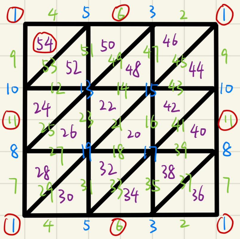
Figure 2: The torus \( {T^{2}} \) , with the opposite edges of the largest square identified.

This simplicial complex has 9 vertices, 27 edges and 18 faces, labelled by integers from 1 to 54. This is viewed as a function \( f \) with image \( \lbrace 1,2,⋯,54\rbrace \) , which can be verified to be a discrete Morse function with 4 critical points encircled in the figure. We describe the gradient field \( V(f) \) : it consists of 25 pairs labelled by \( (i,i+1) \) that do not contain 1, 6, 11, 54. In fact, tracing the numbers in reverse, this is exactly a process that collapses the 25 pairs in order along gradient flow, so that the remaining is a cell complex with one 0-cell, two 1-cells and one 2-cell. As shown by the fundamental theorem, this recovers a cell decomposition of \( {T^{2}} \) . To obtain the homology, we count the gradient flows:

3. From 6 to 1, there are two flows \( 5→4→1 \) and \( 3→2→1 \) that cancel out in orientation.

4. From 11 to 1, there are two flows \( 10→9→1 \) and \( 8→7→1 \) that cancel out in orientation.

5. From 54 to 6, there are two flows \( 53→52→51→50→6 \) and \( 53→52→⋯→39→38→35→34→6 \) that cancel out in orientation.

6. From 54 to 11, there are two flows \( 53→52→⋯→40→11 \) and \( 53→⋯→38→35→⋯→24→11 \) that cancel out in orientation.

It follows that all the boundary maps in the chain complex are zero, hence \( {H_{*}}({T^{2}})={C_{*}} \) and we have the homology groups of the torus:

\( {H_{2}}({T^{2}})≅Z, {H_{1}}({T^{2}})≅Z⊕Z, {H_{0}}({T^{2}})≅Z. \) (72)

6. Conclusion

we gave a survey of both classical Morse theory and discrete Morse theory, and presented their applications. For the classical Morse theory, it can be applied to prove a theorem on the total curvature of knots. For the discrete Morse theory, we applied it to compute the simplicial homology of torus. We outlined the analogies between the two theories entitled "Morse theory", and examined the correspondence of the notions thereof.

References

[1]. István Fáry. Sur lacourbure totaled’une courbe gauche faisant un noeud. Bulletin de la société mathématique de France, 77:128–138, 1949.
[2]. John W Milnor. On the total curvature of knots. Annals of Mathematics, pages 248–257, 1950.
[3]. Anton Petrunin and Stephan Stadler. Six proofs of the fáry-milnor theorem. arXiv preprint arXiv:2203.15137v2, 2023.
[4]. WB Raymond Lickorish. An introduction to knot theory, volume 175. Springer Science & Business Media, 1997.
[5]. Elsa Abbena, Simon Salamon, and Alfred Gray. Modern differential geometry of curves and surfaces with Mathematica. Chapman and Hall/CRC, 2017.
[6]. John W Milnor. Morse theory. Number 51. Princeton university press, 1963.
[7]. Michele Audin, Mihai Damian, and Reinie Erné . Morse theory and Floer homology, volume 2. Springer, 2014.
[8]. John M Lee. Smooth manifolds. Springer, 2012.
[9]. Gerald Teschl. Ordinary differential equations and dynamical systems, volume 140. American Mathematical Soc., 2012.
[10]. Allen Hatcher. Algebraic Topology. Cambridge University Press, 2002.
[11]. Lawrence Craig Evans. Measure theory and fine properties of functions. Routledge, 2018.
[12]. Robin Forman. A user’s guide to discrete morse theory. Séminaire Lotharingien de Combinatoire [electronic only], 48:B48c–35, 2002.
[13]. Arthur B Kahn. Topological sorting of large networks. Communications of the ACM, 5(11):558–562, 1962.
[14]. Nicholas A Scoville. Discrete Morse Theory, volume 90. American Mathematical Soc., 2019.
Cite this article
Dong,Z. (2025). Morse Theory, Discrete Morse Theory and Applications. Theoretical and Natural Science,87,36-51.
Data availability
The datasets used and/or analyzed during the current study will be available from the authors upon reasonable request.
Disclaimer/Publisher's Note
The statements, opinions and data contained in all publications are solely those of the individual author(s) and contributor(s) and not of EWA Publishing and/or the editor(s). EWA Publishing and/or the editor(s) disclaim responsibility for any injury to people or property resulting from any ideas, methods, instructions or products referred to in the content.
About volume
Volume title: Proceedings of the 4th International Conference on Computing Innovation and Applied Physics
© 2024 by the author(s). Licensee EWA Publishing, Oxford, UK. This article is an open access article distributed under the terms and
conditions of the Creative Commons Attribution (CC BY) license. Authors who
publish this series agree to the following terms:
1. Authors retain copyright and grant the series right of first publication with the work simultaneously licensed under a Creative Commons
Attribution License that allows others to share the work with an acknowledgment of the work's authorship and initial publication in this
series.
2. Authors are able to enter into separate, additional contractual arrangements for the non-exclusive distribution of the series's published
version of the work (e.g., post it to an institutional repository or publish it in a book), with an acknowledgment of its initial
publication in this series.
3. Authors are permitted and encouraged to post their work online (e.g., in institutional repositories or on their website) prior to and
during the submission process, as it can lead to productive exchanges, as well as earlier and greater citation of published work (See
Open access policy for details).