1. Introduction

Multiple linear regression, as a classical method, has been widely utilized since entering the 21st century. Nowadays, applications can be found by continuous crossover with other subjects. With its advantages of strong interpretability and high computing efficiency, multiple linear regression is still a core tool for explanatory modeling in data science [1].

For example, multiple linear regression can be closely integrated with the economic field to study and predict a range of consumption and investment activities. Analysis of energy consumption can be seen in Ref. [2]. In this article, authors point out that energy consumption has become a crucial factor for not only users but also manufacturers and policy makers. Through a newly-built energy consumption predicting model based on multiple linear regression, the consumption is forecast with a better reliability, providing valuable information for improving. In Ref. [3], author notices problems of enterprise environmental management. Therefore, a cost benefit estimation method is proposed on basis of multiple linear regression to improve the accuracy and speed of estimation results. In medical field, regression is used as a vital tool as well. To make the cost of medical insurance more reasonable, a prediction method using regression is illustrated [4]. Under ideal circumstances, this model is of great importance in satisfying both public and organizations. Online finance has been a hit in the past several decades, however, a lot of problems exist. By applying multiple linear regression to e-commerce field, authors are able to figure out issues like financing difficulties [5]. What is more, the model can also present some advantages and disadvantages from different perspectives. Cost evaluation is an important method of cost control of power transmission and transformation projects. Through regression analysis, cost evaluation quality can be hugely improved by provided references, allowing for more profitable investments [6].

In this paper, some basic theories of multiple linear regression are introduced at beginning. Then it is followed by a simple example of the previous theories. Examples of applications are also included in the main body part, presenting how various of multiple linear regression models and analysis approaches apply to housing price, medical cost and bank performance respectively. In the end, general characteristics of multiple linear regression can be concluded from a range of perspectives.

2. Method and Theory

2.1. Multiple Linear Regression

Multiple linear regression is widely used as a statistical tool [7]. What really counts is its ability to describe the relationship of a specific dependent variable \( Y \) and multiple independent variables \( {X_{1}}, {X_{2}}, ⋯, {X_{p}} \) . This method can improve simple linear regression by combining multiple variables, allowing for a more complicated and general analysis of the factors influencing the dependent variable. Mathematically, it can be expressed by the following formula

\( Y={β_{0}}+{β_{1}}{X_{1}}+{β_{2}}{X_{2}}+⋯+{β_{p}}{X_{p}}+ε.\ \ \ (1) \)

Variable \( Y \) on the left side of equation is predicted from \( p \) predictor variables \( {X_{1}},{X_{2}},⋯,{X_{p}} \) . The relationship between \( Y \) and \( {X_{1}},{X_{2}},⋯,{X_{p}} \) is linear with coefficients \( {β_{0}} , {β_{1}} ,⋯ \) , \( {β_{p}} \) , and \( ε \) is the error term. The major task is to obtain least squares estimates \( {\hat{β}_{0}},{\hat{β}_{1}},{\hat{β}_{2}},⋯,{\hat{β}_{p}} \) . To do the estimation, one can use matrix to calculate by least squares is a convenient approach.

To illustrate, four matrixes are defined as the ( \( n × 1 \) ) vector \( Y \) , the \( n × (p + 1) \) matrix \( X \) , the \( (p + 1)×1 \) vector unknown regression parameters \( β \) and the \( (n × 1) \) vector \( ε \) random errors like:

\( X=(\begin{matrix}1 & {x_{11}} & ⋯ & {x_{1p}} \\ 1 & {x_{21}} & ⋯ & {x_{2p}} \\ ⋮ & ⋮ & ⋱ & ⋮ \\ 1 & {x_{n1}} & ⋯ & {x_{np}} \\ \end{matrix}),Y=(\begin{matrix}{y_{1}} \\ {y_{2}} \\ ⋮ \\ {y_{p}} \\ \end{matrix}),β=(\begin{matrix}{β_{0}} \\ {β_{1}} \\ ⋮ \\ {β_{p}} \\ \end{matrix}),ε=(\begin{matrix}{ε_{1}} \\ {ε_{2}} \\ ⋮ \\ {ε_{n}} \\ \end{matrix})\ \ \ (2) \)

and \( {e_{i}} \) = random fluctuation (or error) in \( {Y_{i}} \) , i.e.,

\( {Y_{i}}={β_{0}}+{β_{1}}{X_{1i}}+{β_{2}}{X_{2i}}+⋯+{β_{p}}{X_{pi}}+{ε_{i}}.\ \ \ (3) \)

One can define the residual sum of squares (RSS) as

\( RSS=\sum _{i=1}^{n}{{\hat{e}_{i}}^{2}}=\sum _{i=1}^{n}{({y_{i}}-{\hat{y}_{i}})^{2}}\ \ \ (4) \)

Then the residual sum of squares as a function of \( β \) can be written in matrix form as

\( RSS(β)={(Y-Xβ)^{ \prime }}(Y-Xβ)={Y^{ \prime }}Y+{β^{ \prime }}({X^{ \prime }}X)β+{2Y^{ \prime }}Xβ\ \ \ (5) \)

In order to find the least squares estimates, differentiating the formula with respect to \( β \) and equating the result to zero and then canceling out the 2 common to both sides are needed. This gives the following matrix form of the normal equations \( ({X^{ \prime }}X)β={X^{ \prime }}Y \) . The least squares estimates are given by \( \hat{β}={({X^{ \prime }}X)^{-1}}{X^{ \prime }}Y \) .

2.2. Example

Here is a simple example to illustrate the linear regression. Consider a range of samples shown in Table 1, according to Eq. (1), the model can be fitted as \( Y={β_{0}}+{β_{1}}{X_{1}}+{β_{2}}{X_{2}}+ε \) .

Table 1: Data of samples for linear regression.

Below the purpose lies in estimating \( {β_{0}},{β_{1}},{β_{2}} \) . Based on Eq. (2), one can define

\( X=(\begin{matrix}1 & 100 & 2 \\ 1 & 150 & 3 \\ 1 & 200 & 3 \\ 1 & 250 & 4 \\ 1 & 300 & 4 \\ \end{matrix}),Y=(\begin{matrix}300 \\ 400 \\ 500 \\ 600 \\ 700 \\ \end{matrix}),\hat{β}=(\begin{matrix}{\hat{β}_{0}} \\ {\hat{β}_{1}} \\ {\hat{β}_{2}} \\ \end{matrix})\ \ \ (6) \)

The estimates of \( \hat{β} \) come out

\( \hat{β}={({X^{ \prime }}X)^{-1}}{X^{ \prime }}Y=(\begin{matrix}12.8 & -0.08 & -2.4 \\ -0.08 & 0.0008 & 002 \\ -2.4 & 0.02 & 0.6 \\ \end{matrix})(\begin{matrix}2500 \\ 575000 \\ 8850 \\ \end{matrix})=(\begin{matrix}100 \\ 2 \\ -50 \\ \end{matrix})\ \ \ (7) \)

Therefore, results can be shown as \( {\hat{β}_{0}}=100,{\hat{β}_{1}}=2,{\hat{β}_{2}}=-50 \) , and the regression equation can be written as \( Y=100+2{X_{1}}-50{X_{2}} \) .

3. Applications

3.1. Housing Prediction

In the Ref. [8], the authors proposed that previous study has identified three categories of characteristics that have a substantial impact on overall housing prices: house conditions, environmental factors, and transportation considerations.

Spearman's correlation coefficient has been considered as a nonparametric statistical approach to evaluate the monotonic association between two variables. Comparing to Pearson's correlation coefficient, the Spearman's measure of correlation does not require the data to follow a linear connection, giving it a benefit when dealing with nonlinear interactions. Furthermore, Spearman's correlation coefficient is insensitive to extremes and can deal with discontinuous data.

Based on the traditional model, a newly-built linear regression model can be set as:

\( {y_{i}}={β_{0}}+{B^{ \prime }}{x_{i}}+{ε_{i}}\ \ \ (8) \)

where \( {y_{i}}={({x_{i1}},⋯,{x_{id}},⋯,{x_{iD}})^{ \prime }} \) and \( {x_{i}} \) are the \( D \) -dimensional vector of output variables and the \( P \) -dimensional vector of fixed regressor values for \( {i^{th}} \) sample unit correspondingly. \( {β_{0}} \) is a \( D \) -dimensional vector containing the intercepts for \( D \) response. \( B \) is a \( P×D \) vector matrix whose element \( {β_{pd}} \) is the regression coefficient of \( {p^{th}} \) regressor on the \( {d^{th}} \) response. \( {ε_{i}} \) represents the \( D \) -dimensional random vector of the error terms relating to the \( {i^{th}} \) observation. Noticeably, there is an assumption that the multiple linear regression model satisfies the equation

\( {ε_{i}}~\sum _{k=1}^{K}\prod _{k}MVN({ν_{K}},\sum K),\ \ \ (9) \)

with a condition that positive weights \( {π_{k}} \) and \( {ν_{k}} \) are required to gain the relationship \( \sum _{k=1}^{K}{π_{k}}{ν_{k}} \) .

The raw data is then standardized. In the tradition of regression analysis, the complete dataset is separated into two parts: training and testing. By comparing the regression results from the training set to the modeling results from the test set, the model's accuracy and efficiency may be successfully assessed. During the training procedure, the gradient descent optimizer is used to determine the ideal parameters. The progressive fall of the loss function indicates that the parameters in the model are becoming more suited for application.

Afterwards, the trained parameters above are applied to the prediction. The author chooses 100 samples from the dataset for the model. Figure 1 shows an obvious conclusion, indicating that the model's anticipated outcomes are compatible with the trend of the actual values in general, and in the majority of cases, predicted values change in the same direction as the actual values. Some errors occur concurrently, although they are often considered acceptable. It can be inferred that the multiple regression model can forecast and evaluate property prices to a certain degree. However, the prediction has a limited accuracy.

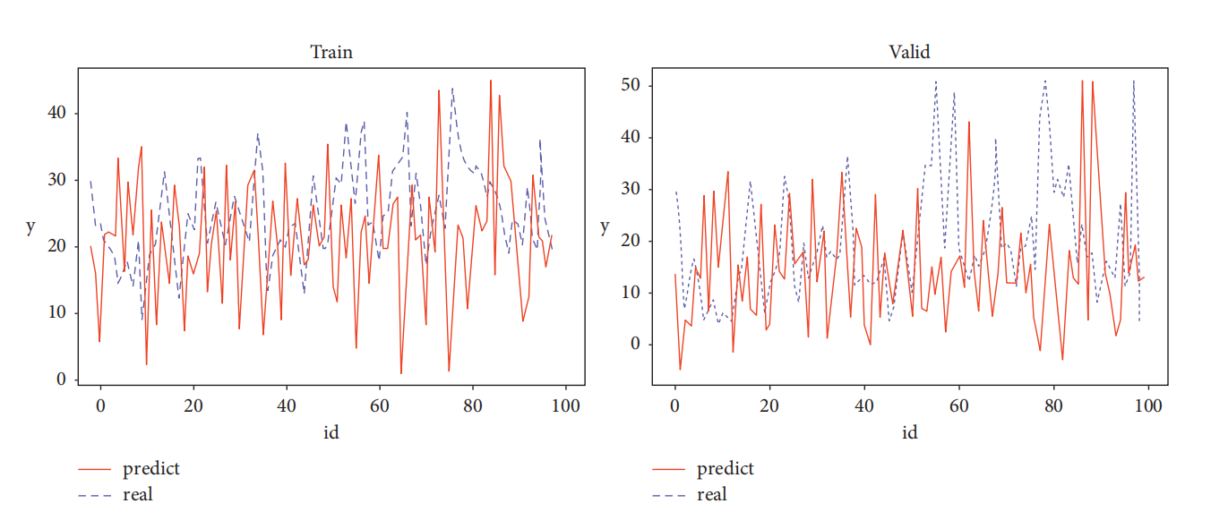
Figure 1: The real and prediction result [8].

3.2. Treatment Cost Prediction

By anticipating the expenditures of disease treatment, some organizations can effectively promote health insurance reform, rationalize medical resource allocation, and reduce patient burdens. In article [9], characteristics influencing treatment costs were collected from the electronic medical record, including the patient's age, gender, surgical history, treatment regimen, previous medical history, current admission status, smoking status, diabetes, and hypertension. The information provided above is divided into four sections: patient explanation, history of current illness, medical history, and personal history. To utilize the data better, preprocess the data is of great significance. Written textual descriptions (e.g., gender, medical history, etc.) in the electronic medical record are translated into numerical variables for use in model calculations.

To make the given data match better, the error term \( ε \) in Eq. (1) may be defined as a variable whose function is setting the coefficients of some low action variables into 0 in the iterative process. Therefore, it possesses the ability to deal with the situation where limited data appear. By comparison, local weighted LASSO (Least Absolute Shrinkage and Selection Operator) regression simplifies the model structure by compressing the coefficients of variables whose impact is relatively small to improve generalization. The specific error term is set as bellow:

\( ε=min\frac{1}{m}[λ\sum _{i=1}^{m}|{β_{i}}|]\ \ \ (10) \)

where \( m \) is the number of samples, \( λ \) is the regularization coefficients, \( {β_{i}} \) is the model parameter. Further, an upper limit is required to make the parameters easier to deal with \( \sum _{i=1}^{n}|{β_{i}}|≤σ \) . One can enlarge or compress \( β \) with the value of \( σ \) changing.

In most cases, random variables represent normal distribution features, so the authors introduced weight function based on normal distribution as \( {ω^{(i)}}=exp(-\frac{{x^{(i)}}-x}{2{σ^{2}}}) \) . Thus, \( ε \) can be written as below, which allows for a local weighted way to promise the efficiency and feasibility of model:

\( ε=min\frac{1}{m}[λ\sum _{i=1}^{m}{ω^{(i)}}{β_{i}}]\ \ \ (11) \)

Then comes the example data analysis. After the preprocess and classification, the data is regressed and fitted for different categories to acquire prediction situation of several models. To illustrate directly, linear regression, LASSO regression, neural network, locally weighted LASSO regression and Bayesian network fusion local weighted LASSO regression are included. Conclusions can be drawn by comparing values like accuracy in Table 2.

Table 2: Comparison of different models in accuracy

From Table 2, accuracy of LASSO regression and Bayesian network fusion local weighted LASSO regression is apparently much higher than the rest of the models, which manifest that locally weighted LASSO regression does have advantages in generalization ability and validity. Furthermore, when combining with Bayesian network classification, the model can gain a more excellent prediction capacity during the experiment. The model is found valid in predicting the expense of treatment for a patient with a limited amount of data and is able to recommend an appropriate treatment plan for the patients.

3.3. Financial Performance of Bank

Banks are of great importance in economic growth, especially private banks. India's banking system has made remarkable achievements over the past few decades, particularly in the areas of risk management and capital adequacy. In order to assess the financial performance of a bank, it is usually analyzed using financial ratios. People also use the financial data of banks for the period 2006 to 2017 to assess banks’ performance through three key indicators and uses multiple regression analysis to develop three models [10].

To begin with, Return on Assets \( (ROA) \) , the ratio of market value of banks to book value of equity ( \( Tobin \prime s Q \) ) and Return on Equity \( (ROE) \) are introduced as three dependent variables. Subsequently, five independent variables \( Bank size \) , Credit Risk \( (CR) \) , Operational Efficiency \( (OE) \) , Asset Management \( (AE) \) , Debt Ratio \( (DR) \) are added as well.

Then, the authors consider the three dependent variables respectively with 3 different models. In each model, a null hypothesis that the single dependent variable is not influenced by the given 5 independent variables is presented. Log of Total Assets (TA) is used to represent \( Bank size \) . Total debt/TA represents Debt Ratio. Afterwards, do the multiple linear regression analysis and hypothesis test through calculated data.

In the first model, the regression model can be assumed as:

\( ROA={β_{0}}+{β_{1}}CR+{β_{2}}OE+{β_{3}}AM+{β_{4}}Bank size+{β_{5}}DR+ε\ \ \ (12) \)

The analysis results are presented in Table 3.

Table 3: Coefficients of the first model

The ANOVA (Analysis of Variance) result of the first model indicates that null hypothesis against alternative hypothesis. If the specific variable's Significance level is less than 0.05, it is assumed that the predictor variables do not have a significant impact on relevant variable in the model. Therefore, CR, OE and AM have significant influence on \( ROA \) while \( Bank size \) and Debt Ratio’s impact on \( ROA \) is not apparent. In the second model, the regression model is the equation as below:

\( Tobi{n^{ \prime }}s Q={β_{0}}+{β_{1}}CR+{β_{2}}OE+{β_{3}}AM+{β_{4}}Bank size+{β_{5}}DR+ε\ \ \ (13) \)

The analysis results are shown in Table 4.

Table 4: Coefficients of the second model

After doing the ANOVA, it can be seen that the null hypothesis against alternative hypothesis. The observed significance level (p-value) provides empirical evidence that the model achieves statistical significance at the predetermined 5% threshold. Therefore, from Table 4, on one hand, \( Bank size \) and DR have significant impact on \( Tobin \prime s Q \) . On the other hand, the rest 3 variables show insignificant effect on \( Tobin \prime s Q \) .

In the third model, authors consider the model as:

\( ROE={β_{0}}+{β_{1}}CR+{β_{2}}OE+{β_{3}}AM+{β_{4}}Bank size+{β_{5}}DR+ε\ \ \ (14) \)

The analysis results can be seen from Table 5.

Table 5: Coefficients of the third model.

Results can be seen from ANOVA of the third model that null hypothesis against alternative hypothesis. The significance of variables can be evaluated from Significance Level in Table 5 respectively, which indicates CR, AM and \( Bank size \) have significant influence on \( ROE \) . OE and DR have insignificant impact on \( ROE \) . Ultimately, the three models above derive the key factors affecting their financial performance, which provide a comprehensive view of the bank's operations and risk levels for bank managers and investors.

4. Conclusion

Considering the results, it is natural to find that multiple linear regression is a flexible method when combining with other techniques like neural network and Bayesian network. What really counts is that its massive potential value has been shown significant in numerous areas. The model is easy to understand and express because its coefficients visualize the relationship between the variables directly. By quantifying the effects of each factor, multiple linear regression can be clearly accomplished in complex scenarios, adapting to the needs of modern data analysis. However, it is not always the perfect choice in many circumstances. Due to its strict hypothesis, realistic data usually fail to meet the conditions of independent and identical distribution and linear relationship. What’s more, some abnormal data may do extreme harm to the whole model, resulting in error and irrational consequences. This paper is limited in presenting the process of building the model specifically. In addition, some preprocessing of the selected data is neglected. For further development, future research may focus on how multiple linear regression can better connected with other powerful tools and deal with data whose relationship with other factors is nonlinear. When combining with artificial intelligence, the modeling process may be optimized automatically, lowering the expenditure and time consumption on adjusting the given environments.

References

[1]. Montgomery, D. C., Peck, E. A., & Vining, G. G. (2021). Introduction to linear regression analysis. John Wiley & Sons.
[2]. Chen, Y., Huang, M., & Tao, Y. (2022). Density-based clustering multiple linear regression model of energy consumption for electric vehicles. Sustainable Energy Technologies and Assessments, 53, 102614.
[3]. Wang, M. (2025). Study on cost benefit estimation of enterprise environmental management based on multiple linear regression. International Journal of Manufacturing Technology and Management, 39(1/2), 74-88.
[4]. Alzoubi, H. M., Sahawneh, N., AlHamad, A. Q., Malik, U., Majid, A., & Atta, A. (2022, October). Analysis of cost prediction in medical insurance using modern regression models. In 2022 International Conference on Cyber Resilience (ICCR) (pp. 1-10). IEEE.
[5]. Wang, P., & Han, W. (2021). Construction of a new financial E-commerce model for small and medium-sized enterprise financing based on multiple linear logistic regression. Journal of Organizational and End User Computing (JOEUC), 33(6), 1-18.
[6]. Ye, M., Chen, X., Chen, K., Liu, M., & Wu, H. (2023, March). Research on cost evaluation of power transmission and transformation project based on grey correlation and regression analysis. In Second International Conference on Statistics, Applied Mathematics, and Computing Science (CSAMCS 2022) (Vol. 12597, pp. 1049-1054). SPIE.
[7]. Aiken, L. S., West, S. G., Pitts, S. C., Baraldi, A. N., & Wurpts, I. C. (2012). Multiple linear regression. Handbook of Psychology, Second Edition, 2.
[8]. Zhang, Q. (2021). Housing price prediction based on multiple linear regression. Scientific Programming, 2021(1), 7678931.
[9]. Tong, L. L., Gu, J. B., Li, J. J., Liu, G. X., Jin, S. W., & Yan, A. Y. (2021). Application of Bayesian network and regression method in treatment cost prediction. BMC Medical Informatics and Decision Making, 21, 1-9.
[10]. Nataraja, N. S., Chilale, N. R., & Ganesh, L. (2018). Financial performance of private commercial banks in India: multiple regression analysis. Academy of Accounting and Financial Studies Journal, 22(2), 1-12.
Cite this article
Jiang,R. (2025). Multiple Linear Regression in Financial Prediction and Evaluation. Theoretical and Natural Science,100,130-136.
Data availability
The datasets used and/or analyzed during the current study will be available from the authors upon reasonable request.
Disclaimer/Publisher's Note
The statements, opinions and data contained in all publications are solely those of the individual author(s) and contributor(s) and not of EWA Publishing and/or the editor(s). EWA Publishing and/or the editor(s) disclaim responsibility for any injury to people or property resulting from any ideas, methods, instructions or products referred to in the content.
About volume
Volume title: Proceedings of the 3rd International Conference on Mathematical Physics and Computational Simulation
© 2024 by the author(s). Licensee EWA Publishing, Oxford, UK. This article is an open access article distributed under the terms and
conditions of the Creative Commons Attribution (CC BY) license. Authors who
publish this series agree to the following terms:
1. Authors retain copyright and grant the series right of first publication with the work simultaneously licensed under a Creative Commons
Attribution License that allows others to share the work with an acknowledgment of the work's authorship and initial publication in this
series.
2. Authors are able to enter into separate, additional contractual arrangements for the non-exclusive distribution of the series's published
version of the work (e.g., post it to an institutional repository or publish it in a book), with an acknowledgment of its initial
publication in this series.
3. Authors are permitted and encouraged to post their work online (e.g., in institutional repositories or on their website) prior to and
during the submission process, as it can lead to productive exchanges, as well as earlier and greater citation of published work (See
Open access policy for details).