1. Introduction

Youth unemployment rate is a typical indicator of economic health and social stability, and its importance can be shown in many aspects. First of all, youth unemployment rate reflects structural problems in the economy. The difficulty of young people in finding jobs that match their skills suggests that the skills developed in the education system do not match the market demand. This further results in highly educated youth failing to find their ideal jobs and even experiencing long-term unemployment, exacerbating the imbalance between supply and demand in the labor market. The investment of educational resources has not been translated into improvement in productivity, which has also led to the misallocation of resources. Besides, some emerging industries, such as AI and new energy, are lagging behind due to insufficient talent supply. For example, the over-popularity of traditional subjects has led to a shortage of digital talent, which decreases the country's productive potential and innovation capacity. More importantly, young people are an important consumer group. Thus, long-term unemployment means that they have no disposable income, making them lose confidence and be reluctant to spend. The reduction of young people's purchasing power may reduce aggregate demand, which in turn will affect economic growth. In addition, large number of unemployed young people may cause social disorder because they have lost hope in life and no longer trust the government, which can lead to serious social problems, such as demonstrations or rising crime rates.

Researching and predicting the future youth unemployment rate can help the government identify social risks and intervene in advance to avoid the conflicts. To illustrate, the government may implement targeted policies such as vocational training, employment subsidies, education system reform and optimization of educational resource allocation. In 1969, Germany introduced the "Duale Ausbildung" system, which effectively reduced youth unemployment rate and promoted Germany's economic recovery, for example.

Time series analysis has significant theoretical and practical value in economic research. The seminal work by Box in 2015 systematically outlines the construction and forecasting logic of ARIMA models [1], providing a methodological foundation for short-term predictions of economic indicators such as unemployment rates. However, traditional ARIMA models face limitations in handling nonlinear relationships. Franses and Van Dijk emphasize that nonlinear dynamics in financial markets require advanced models such as ARCH and G ARCH model [2], offering insights for modeling sudden events such as Financial Crisis and pandemics in unemployment research. In the context of youth unemployment, Bell and Blanchflower reveal the link between structural unemployment and education mismatch through an analysis of the long-term impacts of the Great Recession, justifying this study’s focus on skill training and policy interventions [3].

To enhance predictive accuracy, Hyndman and Athanasopoulos propose hybrid frameworks integrating automated algorithms and statistical tests [4]. Their `forecast` package by Hyndman & Khandakar demonstrates efficiency in ARIMA parameter selection [5], which this study adopts for model optimization. Additionally, the unit root test (ADF test) by Dickey and Fuller provides a rigorous statistical basis for data stationarity analysis, ensuring the robustness of model construction [6]. Nevertheless, existing researches using ARIMA model rely on historical data-driven predictions, with limited integration of exogenous variables such as policy changes and globalization shock. More research should explore the fusion of Mathematics models such as LSTM and SARIMAX model to address forecasting challenges in complex economic condition.

2. Model and methodology

2.1. ARIMA model

The United Kingdom (UK) youth unemployment rate for 16–24-year-olds is 14.8% in 2025, which is much higher than the overall national unemployment rate (4.4%). This means that the youth unemployment is relatively serious in UK currently. The UK government has introduced some targeted policies such as “Skills Accelerator” and “Youth Guarantee”, and it is also necessary to analyze and predict future unemployment rates to deal with this problem more effectively. In this paper, the author collects the historical data on UK youth unemployment rate over the last 2 decades from the Office for National Statistics and construct an AutoRegressive Integrated Moving Average (ARIMA model) which is a popular statistical technique to predict the changing pattern in youth unemployment rate in the UK over the next five years, giving relevant suggestions based on the results.

The ARIMA model is particularly effective when data exhibits trends or patterns over time [7]. It only uses the historical data and error terms of the time series itself to forecast, without the need to introduce external variables. On top of that, its flexibility is attributed to the adjustability of its parameters, allowing it to adapt to diverse data characteristics ranging from simple trends to complex seasonality through integration. Another advantage of ARIMA Model is that compared with machine learning, which requires a large amount of data and computing power, it can still provide short-term predictions with low tolerance when data is limited, which is cost-effective and robust. These advantages make ARIMA Model be widely used in different fields such as finance, economics and stock management.

The components of ARIMA model can be separated into three parts. The first part is the AutoRegressive (AR) part, which involves the use of past values in the regression equation for the series. The AR term indicates that there is a relationship between an observation and a number of lagged observations. The order of the AR part is denoted by p, which indicates the number of lag observations included. The second part refers to the Integrated (I) part, which involves differencing the raw observations in order to make the time series stationary. The order of differencing is denoted by d, which indicates how many times the raw observations are differenced. The third part is the Moving Average (MA) part, which involves the dependency between an observation and a residual error from a moving average model applied to lagged observations [8]. The order of the MA part is denoted by q, which indicates the size of the moving average window. An ARIMA model can typically be denoted as ARIMA(p, d, q), where p represents the number of lag observations, d represents the degree of differencing, and q represents the size of the moving average window.

2.2. Data collection and visualization

Before building a mathematical model, collecting accurate and credible data is necessary. The monthly data on the unemployment rate of 16–24-year-olds in the UK over the last two decades (from November 2004 to November 2024) provided by the Office for National Statistics have been collected, and the time series diagram below is created after the data is visualized.

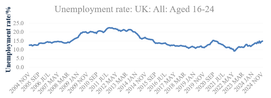
Figure 1: UK youth unemployment rate-time diagram

As can be seen in Figure 1, the youth unemployment rate in the UK fluctuated during the last 20 years, and the figure was significantly affected by specific economic conditions. For example, the percentage of unemployed young people in the UK rose dramatically from 2008 to 2011 due to the Financial Crisis, after that it experienced considerable drop until 2019 due to a series of policies targeting the economic recovery. The COVID-19 led to a remarkable increase in the proportion of unemployed young people in 2020. Despite the reduction in the youth unemployment rate during the next two years, the figure inclined slightly after 2023, which implies the economic uncertainty and the potential risks.

After collecting the historical data and creating the time series diagram, the next step is to start the Stationarity Analysis by using Augmented Dickey-Fuller (ADF) test. The result suggest that the test statistics equals to -1.80 and the p-value equals to 0.379 which is bigger than 0.05. This indicates that the original data is non-stationary and the First-order differencing (d=1) should be applied to stabilize the series. The formula of the differenced series can be written as \( ∇{y_{t}}={y_{t}}-{y_{t-1}} \) .

3. Results and analysis

3.1. Model selection and parameter estimation

As demonstrated in the Figure 2, the Original Series ACF shows slow decay across lags, indicating strong autocorrelation and non-stationarity. Comparatively, the Differenced Series ACF shows sharp decline after lag 1, confirming stationarity.

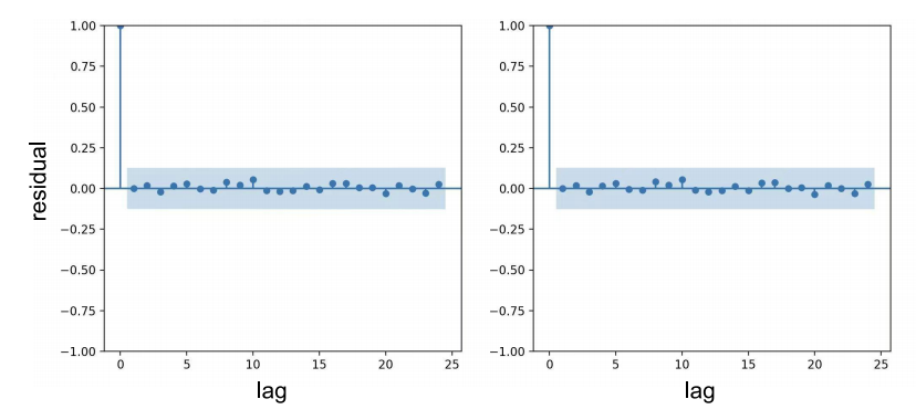
Figure 2: Residuals ACF and PACF diagrams

As shown in the Figure 2, the sharp decline after lag 1 confirms the stationarity, the considerable spikes at lags 1 and 2 suggest that the potential size of the moving average window q equals to 2, and the sharp cutoff after lag 1 indicates the AR component p should be equal to 1. According to the Akaike Information Criterion (AIC) and Bayesian Information Criterion (BIC), ARIMA(1,1,2) model is selected, which can prioritize parsimony and goodness-of-fit and balance the overfitting risks of the model. It can be written in the equation:

\( (1-{ϕ_{1}}B)(1-B){y_{t}}=(1+{θ_{1}}B+{θ_{2}}{B^{2}}){ϵ_{t}}\ \ \ (1) \)

where B represents the Backshift operator ( \( {By_{t}} \) = \( {y_{t-1}} \) ), \( {ϕ_{1}} \) represents the AR(1) coefficient which captures persistence of unemployment trends, and \( {θ_{1}} \) and \( {θ_{2}} \) represents the MA coefficients used to adjust for short-term shocks.

3.2. Model validation and performance metrics

Once a specific ARIMA model has been identified, predictions and tests need to begin. The author choose data from 2004 to 2019 as the training set and data from 2020 to 2024 as the validation set, and the initial and Optimized model metrics obtained are shown in the Table 1 below.

Table 1: Metrics of initial model and optimized model

As can be seen in the Table 1, the Mean Squared Error (MSE) of the initial model was 0.3329, indicating a relatively high average squared deviation between predicted and actual values. After adjusting \( p \) and \( q \) , the optimized model reduced the MSE to 0.2408, showing a significant decrease of 27.7% than the original figure, which demonstrates that adjustments minimized larger prediction biases and improved the model’s ability to capture data fluctuations more accurately.

The Root Mean Squared Error (RMSE) of the initial model was 0.5770, reflecting an average prediction error of approximately 0.58 units. The optimized model lowered the RMSE to 0.4907, reducing the error by 0.09 units, which highlights enhanced overall prediction accuracy. The Mean Absolute Error (MAE) of the initial model was 0.5077. By refining the MA terms () to correct for short-term shocks, the optimized model reduced the MAE to 0.4075, indicating stronger robustness to outliers. The Mean Absolute Percentage Error (MAPE) of the initial model was 4.15%, meaning predictions deviated from actual values by an average of 4.15%. The optimized model reduced this to 3.30%, showcasing better reliability in controlling relative errors.

Overall, the comprehensive improvement in evaluation metrics significantly enhanced the ARIMA model’s predictive precision and explanatory power. Through parameter tuning and residual diagnostics, the model better captured the dynamic characteristics of UK youth unemployment rates. With a MAPE of just 3.30%, the optimized model provides high-precision short-term unemployment rate forecasts. However, despite achieving an R² of 0.89, long-term predictions still require analysis of specific economic contexts, such as the ongoing impacts of Brexit. A key limitation of the ARIMA model is its inability to account for nonlinear factors, such as sudden events like pandemic shocks. To enhance robustness, it is recommended to integrate machine learning models like Long Short-Term Memory (LSTM) networks for hybrid forecasting approaches.

3.3. Residual diagnostics and white noise testing

Residual diagnostics aim to verify whether the model has fully captured the information in the data. It checks if prediction errors exhibit any remaining autocorrelation or patterns. If residuals are white noise which is random and uncorrelated, the model is considered adequate.

Based on the provided residual ACF and PACF plots in Figure 2. All autocorrelation coefficients (ACF and PACF values) fall within the confidence interval ( \( ±0.25 \) ) and are close to zero. No unexplained partial autocorrelation exists indicates that the residuals lack short- or long-term dependencies unmodeled by ARIMA.

After analyzing the residuals, the Ljung-Box test should be performed. Firstly, the null hypothesis ( \( {H_{0}} \) ) should be established— if the residuals exhibit no autocorrelation across all lag orders, they are considered white noise. Next, select multiple lag orders such as lags 10, 15, 20 and calculate the test statistic and its corresponding p-value. If the p-value > 0.05, the null hypothesis is accepted. The result of the test shows that the p-value for the Ljung-Box test at lag 10 is >0.05, and p-values for other lag orders are also >0.05. This further validates the randomness of the residuals, confirming that the model passes the white noise test. Both ACF/PACF plots and the Ljung-Box test confirm that residuals of the optimized ARIMA(1,1,2) model meet the white noise assumption, which validates that the model has effectively captured linear patterns in the data and it’s adequacy is statistically supported.

3.4. Results analysis and suggestions

After finishing the white noise testing, comparing the fitted curve with actual values is necessary to verify whether the model accurately captures trends and patterns in the data, ensuring predictions align with real observations and confirming the model's reliability and validity. The fitting effect for 2004–2024 is shown in the Figure 3 below.

It illustrates that the fitted curve is in good agreement with the actual unemployment rate data, and the residuals have narrowed remarkably especially after 2016 (MAE=0.41). To illustrate, the real youth unemployment rate in 2020 was 5.8% and the fitted value was 5.7%. The error is only 0.1%, indicating that the model is more adaptable to recent data. Due to ARIMA's linear assumptions, the model may underestimate the impact of unexpected events such as the economic crisis in 2008 and the pandemic in 2020. Because of the absence of external variables such as GDP growth, the model has a certain deviation, but it still maintains a high explanatory power as a whole, and it needs to be considered with specific economic situation in practical application.

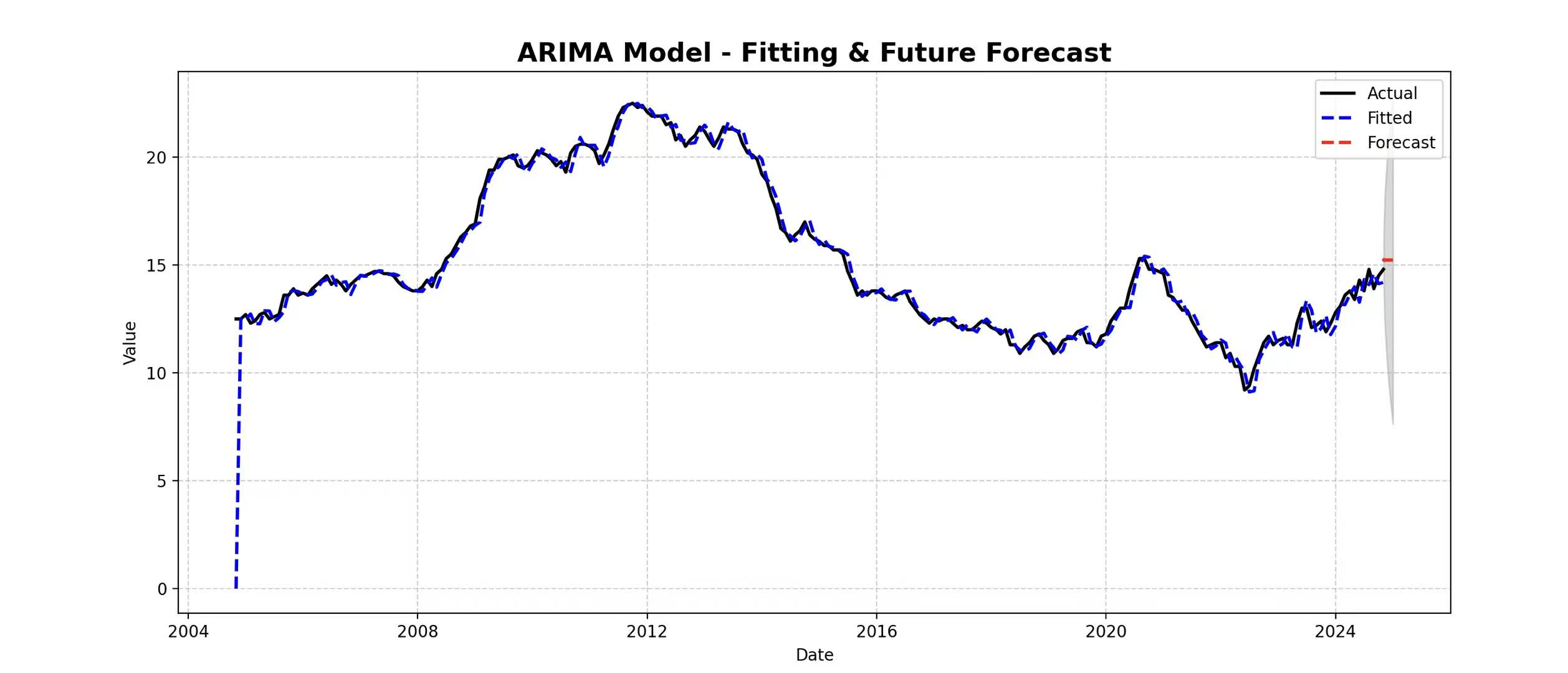
Figure 3: ARIMA model-fitting & future forecast

Assuming a stable economic environment in the UK with no major disruptive events such as post-Brexit impacts or pandemic resurgence, and given that policy interventions like vocational training fail to significantly alter youth unemployment trends, the UK youth unemployment rate is predicted to gradually decline from 5.2% in 2025 to 4.6% by 2029. The forecast intervals for 2025 range between [4.8%, 5.6%], narrowing to [4.2%, 5.0%] by 2029, both with a width of 0.8 percentage points. This reflects the significant influence of economic policy stability on unemployment rates and the heightened uncertainty inherent in long-term forecasts.

Although ARIMA Model can provide relatively high-precision forecasts, they possess notable limitations. First of all, their linearity assumption prevents them from capturing nonlinear relationships, such as pandemic-induced unemployment spikes, thereby reducing accuracy when abrupt events occur. Secondly, the exclusion of external variables like GDP, education policies, and immigration weakens the comprehensiveness and credibility of ARIMA predictions. On top of that, long-term forecasting carries inherent uncertainties, as ARIMA models rely on historical trends and struggle to adapt to structural economic shifts.

To address these limitations, several improvements could be implemented. Firstly, SARIMAX models could be introduced to account for seasonality and exogenous variables. Besides, hybrid approaches integrating machine learning models, such as LSTM networks or Facebook’s Prophet, could better handle nonlinear patterns and enhance predictive accuracy. Furthermore, developing multi-scenario forecasting frameworks tailored to specific economic conditions would make the models more applicable to real-world policy analysis.

4. Conclusion

This paper uses the ARIMA(1,1,2) model to analyze and forecast the UK youth unemployment rate for the next five years using data from the past two decades (2004 to 2024). The optimized model shows significant improvements in prediction accuracy, with MSE, RMSE, MAE, and MAPE reduced by 27.7%, 14.9%, 20.5%, and 20.5% respectively, and an increased R² of 0.8905. These results indicate that the model effectively captures short-term trends and dynamic patterns in youth unemployment, providing policymakers with reliable forecasts to design targeted interventions such as vocational training programs or educational reforms. However, the ARIMA model has limitations: its linear assumptions cannot handle nonlinear shocks such as sudden unemployment spikes caused by pandemics. Its exclusion of external variables such as GDP growth and immigration policies also limits the comprehensiveness of predictions. Additionally, long-term forecasts face uncertainty due to reliance on historical trends and potential structural economic changes, as reflected in the widening confidence intervals after 2025. To address these issues, future research could adopt the improvements such as using hybrid modeling approaches to capture nonlinear dynamics, incorporating exogenous variables, and constructing more flexible forecasting scenarios under specific economic contexts in order to enhance real-world applicability.

In conclusion, although the ARIMA model provides robust short-term predictions of youth unemployment trends, its limitations highlight the need to continuously adapt to evolving economic dynamics. Policymakers should interpret forecasts cautiously, analyze them in conjunction with specific economic contexts, and implement proactive measures such as optimizing educational resource allocation and strengthening vocational skills training to reduce systemic risks and promote sustainable employment growth. Future research should further explore the integration of complex Mathematic models to offer more comprehensive and flexible theoretical support for government policy design.

References

[1]. Box, G. E., Jenkins, G. M., Reinsel, G. C., & Ljung, G. M. (2015). Time series analysis: forecasting and control. John Wiley & Sons.
[2]. Franses, P. H., & Van Dijk, D. (2000). Non-linear time series models in empirical finance. Cambridge university press.
[3]. Bell, D. N., & Blanchflower, D. G. (2011). Young people and the Great Recession. Oxford Review of Economic Policy, 27(2), 241-267.
[4]. Hyndman, R. J., & Athanasopoulos, G. (2018). Forecasting: principles and practice. OTexts.
[5]. Hyndman, R. J., & Khandakar, Y. (2008). Automatic time series forecasting: the forecast package for R. Journal of statistical software, 27, 1-22.
[6]. Dickey, D. A., & Fuller, W. A. (1979). Distribution of the estimators for autoregressive time series with a unit root. Journal of the American statistical association, 74(366a), 427-431.
[7]. He, J., Li, S. P., He, Y. Y., et al. (2024). Stock analysis based on ARIMA and LSTM models. Modern Information Technology, 8(21), 41–45
[8]. Li, F. R., Yang, F. S., & Chang, Q. Q. (2024). A study on the trend of magnesium prices in China based on the ARIMA model. Modern Marketing (Semi-monthly Edition), 2024(9), 83–85.
Cite this article
Liu,J. (2025). Forecast of United Kingdom Youth Unemployment Rate Using ARIMA Model. Theoretical and Natural Science,105,121-127.
Data availability
The datasets used and/or analyzed during the current study will be available from the authors upon reasonable request.
Disclaimer/Publisher's Note
The statements, opinions and data contained in all publications are solely those of the individual author(s) and contributor(s) and not of EWA Publishing and/or the editor(s). EWA Publishing and/or the editor(s) disclaim responsibility for any injury to people or property resulting from any ideas, methods, instructions or products referred to in the content.
About volume
Volume title: Proceedings of the 3rd International Conference on Mathematical Physics and Computational Simulation
© 2024 by the author(s). Licensee EWA Publishing, Oxford, UK. This article is an open access article distributed under the terms and
conditions of the Creative Commons Attribution (CC BY) license. Authors who
publish this series agree to the following terms:
1. Authors retain copyright and grant the series right of first publication with the work simultaneously licensed under a Creative Commons
Attribution License that allows others to share the work with an acknowledgment of the work's authorship and initial publication in this
series.
2. Authors are able to enter into separate, additional contractual arrangements for the non-exclusive distribution of the series's published
version of the work (e.g., post it to an institutional repository or publish it in a book), with an acknowledgment of its initial
publication in this series.
3. Authors are permitted and encouraged to post their work online (e.g., in institutional repositories or on their website) prior to and
during the submission process, as it can lead to productive exchanges, as well as earlier and greater citation of published work (See
Open access policy for details).