1. Introduction

The planet is experiencing a progressively evident warming trend, and this is intensifying extreme weather events and increasing the complexity of the climate system. Observational records in the United Kingdom likewise reveal a warming climate trend [1]. In the capital of the United Kingdom, fluctuations and anomalies in winter temperature are directly related to energy use, traffic safety, and the health of London residents. Therefore, the demand for predicting daily average temperatures in metropolises during the coldest month is of growing importance.

Recent literature on climate research can be mainly classified into two categories. The first concentrates on long-term trend analysis. Researchers in this strand frequently employ statistical modeling approaches (e.g., Generalized Additive Models) to decipher the urban heat island effect, focusing on the trajectory of regional warming across monthly and annual scales. At the same time, the other category focuses on short-term weather prediction. A majority of studies in this strand integrate models such as ARIMA, SARIMA, and hybrid methods, using more complicated machine learning techniques for forecasting temperatures at an hourly scale [2]. Recent work, such as the study done by Khan, S., Ahmed, N., & Ali, R. , has examined daily weather prediction using both statistical and machine learning models [3]. However, few studies systematically compare simple baseline models (such as the mean method and the drift method) with diverse statistical approaches on the same continuous and long-span time series. In addition, research on daily temperature prediction often lacks statistical significance testing to ensure the credibility of the experiment. This limitation poses a barrier to the robust evaluation of model performance and interpretability. Against this background, this article constructs an integrated comparative framework that incorporates conventional mean methods, linear regression methods, and statistical modeling approaches.

This study aims to evaluate the effectiveness of multiple forecasting approaches for predicting urban temperatures under global warming. The contribution of this work can be outlined in four aspects. Firstly, this article conducts a systematic comparison of nine forecasting methods, ranging from mean-based baselines to trend modeling and statistical learning models such as SARIMA, GAM, and ARIMAX. Next, by setting 1979–2019 as the training period and 2020 as an independent test set, the study provides a comprehensive assessment of out-of-sample predictive ability. Third, the study complements the main results with additional diagnostics, including expanding and rolling-window cross-validation, residual analysis, and statistical significance tests (DM test and paired t-test). Finally, from a climatological perspective, an OLS regression is used to identify the long-term warming trend in January mean temperatures in London over the past four decades.

2. Data and experimental design

The data source for this research is the “London Weather” dataset on Kaggle, which supplies a variety of meteorological observations from January 1979 to the end of 2020 in London, including mean temperature, cloud cover, and precipitation [4]. This study mainly focuses on the mean temperature series, since the objective is the January 2020 daily mean temperature estimation. The data from 1979 to 2019 were used for training models, while the 2020 data were left for testing and assessing performance.

2.1. Data processing

The data cleaning procedure followed the typical approach in time-series studies outlined by Hyndman and Athanasopoulos in FPP3 [5]. Initially, the date field was converted into a year–month–day structure and set as the index variable, utilizing the tssible package in R [5]. The year and month components were then extracted for the next step's filtering at the monthly and yearly levels. An additional quality check revealed 36 missing values in the mean_tem column, which were excluded directly from the analysis in this study. The dataset remained unchanged except for this correction for consistency and comparability.

2.2. Forecasting methods

2.2.1. Historical daily mean

Shah I, Mubassir P, Ali S, and Albalawi O highlighted that it is vital to compare baseline and more advanced models in short-term weather prediction [6]. This research firstly applied the historical mean method following this framework, using the average temperature of each January day from 1979 to 2019 to predict values for January 2020:

$$$ \begin{array}{c}{\widehat{y}}_{2020,d}=\frac{1}{N}{\sum }_{t\in T}{y}_{t,d},\hspace{1em}\text{w}\text{h}\text{e}\text{r}\text{e}T=\{\mathrm{1979,1980},\dots ,2019\},\end{array}$$$(1)

where  $$ {\mathrm{x}}_{\mathrm{t},\mathrm{d}}$$  is the observed temperature on day d =1, 2...,31 of year t, N=41.

2.2.2. Filtered mean

This method omits the five hottest and coldest years to reduce the impact of extremes, then adopts the mean method with the remaining 31 years.

2.2.3. Seasonal drift

The framework of the seasonal drift method in this article incorporates the approaches discussed in FPP3 [5]. For each day in January 2020, this model estimates how much that day’s temperature had changed from 1979 to 2019, then extends that trend forward by one more year.

2.2.4. Average yearly linear trend

The average of the yearly linear trend method fits a linear trend to each year’s January temperatures (1979–2019), then averages the slopes and intercepts across years to obtain an overall trend, which is used to forecast January 2020.

2.2.5. Two-Stage trend regression

The Two-Stage trend regression decomposes the forecasting process into two steps, inspired by the Two-Stage strategy outlined by Xu, Q., Wen, Q., and Sun, L. in 2021 [7]. The experiment performed a linear trend fitting to each year’s January temperatures (1979-2019), then regressed the slopes and intercepts on year to capture their evolution. Using the 2020 predicted parameters, the temperature line for January 2020 was reconstructed.

2.2.6. ARIMA

This method concatenates all January daily mean temperature records from 1979 to 2019 into a single time series, then uses the auto.arima function in the forecast package to choose the optimal ARIMA(p, d, q) parameters automatically [8]. Based on the best-fitting ARIMA model, this method derives the forecasted January 2020 values.

2.2.7. SARIMA + typical day reconstruction

A SARIMA model was fitted to monthly mean temperatures (all months, 1979–2019) to capture long-term seasonal patterns in this experiment:  $$ {\widehat{m}}_{\mathrm{2020,1}}=$$  monthly SARIMA forecast (Jan 2020 mean), since SARIMA exhibits strong predictive capability for seasonal weather time series noted by Szostek [9]. The predicted January 2020 mean was then combined with daily deviations computed by the mean method to generate forecasts.

2.2.8. GAM

Similar to Bassett et al., whose study employed the Generalized Additive Model (GAM) to analyze the UHI trends in London, this research also applied the GAM to capture the non-linear relationships in January temperatures [10].

2.2.9. ARIMAX (dynamic regression)

The study fitted an ARIMAX (dynamic regression) model incorporating a linear trend and Fourier terms as external predictors, together with ARIMA errors. Following the procedures described in FPP3, this method is used to forecast January 2020 daily temperatures [5].

2.3. Evaluation metrics

The accuracy of each model in this study is evaluated against the observed temperature by Mean Absolute Error (MAE) and Root Mean Squared Error (RMSE). MAE measures the average magnitude of distance between predictions and reality, while RMSE penalizes significant prediction errors through squaring the deviation before computing the mean. MAE and RMSE are widely accepted metrics in meteorological model performance assessment, as Chai and Draxler noted in 2014 [11]. The mathematical definitions of MAE and RMSE are expressed as:

$$$ \begin{array}{c}\text{M}\text{A}\text{E}=\frac{1}{n}{\sum }_{i=1}^n\left|y_i-\widehat{y_i}\right|,\end{array}$$$(2)

$$$ \begin{array}{c}\text{R}\text{M}\text{S}\text{E}=\sqrt{\frac{1}{n}{\sum }_{i=1}^n{\left(y_i-\widehat{y_i}\right)}^2},\end{array}$$$(3)

where  $$ y_i$$  represents the observed value,  $$ \widehat{y_i}$$  denotes the predicted value, and n is the number of observations.

2.4. Cross-validation procedures

To assess predictive performance, this study employed two cross-validation strategies: expanding window CV (cross-validation) and rolling window CV, following the practice of time-series forecasting for pipelines conducted by Meisenbacher in 2022 [12]. The expanding window CV in this research progressively incorporates additional historical data with a minimum 20-year window, showing how forecasting capability improves with more information. In comparison, the 20-year and 30-year rolling window CV reflects the adaptability to recent data.

2.5. Statistical significance tests

This research conducted Diebold–Mariano test (Diebold & Mariano, 1995) and the paired t-test to assess the statistical significance of prediction performance differences between the three top-performing models [13]. The first statistical test, the DM test, is designed to compare two models and evaluate whether one forecasting method significantly outperforms another in terms of predictive accuracy at the daily level. The paired t-test concentrates on variations in annual average errors, highlighting the overall performance in a relatively long period. The application of both tests offers a more comprehensive evaluation.

3. Results

3.1. Forecasting accuracy

The accuracy is assessed using the London January 2020 mean temperature dataset, and the models were trained using the record of daily average temperatures from 1979 to 2019. The Two-Stage trend regression is the top performer (MAE = 2.33 °C; RMSE = 2.74 °C; Table One) among all nine different methods, and the Filtered Mean method and SARIMA + Typical Day Reconstruction show similar performance on MAE and RMSE (2.63/3.14 °C and 2.64/3.15 °C, respectively). Compared with the Filtered Mean method, Two-Stage trend regression reduces the error by 0.30 °C in MAE (approximately 11.6%) and 0.41 °C in RMSE (approximately 13%). A discernible gap can be seen between the top three best-performing approaches and the fourth-best model (GAM), which is approximately 0.19 °C in MAE and 0.18 °C in RMSE.

As shown in Figure 1, it visualizes the actual daily average temperature curve alongside predicted trajectories. Two-Stage tracks the slow within-month trend while preserving the overall level. In contrast, the Filtered Mean method and SARIMA+Typical Day Reconstruction remain close to the climatological daily pattern, but they cannot capture the intra-month drop in heat. The Historical Daily Mean model (MAE ≈ 2.87 °C) is competitive, while it is clearly behind the top performers. The ARIMA model on the stacked January continuous time series yields a forecast of a random walk (ARIMA (0, 1, 0)), with a high MAE value (7.95 °C), suggesting mis-specification for this structure. ARIMAX improves upon ARIMA but remains inferior to trend-aware linear regression models or climatology-based simple baselines.

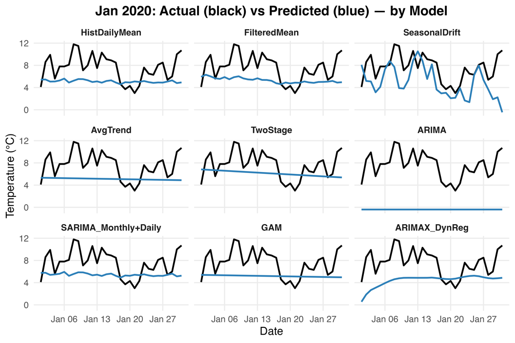
Overall, models that incorporate inter-annual trend information or robust January climatology achieve the strongest accuracy on this task.

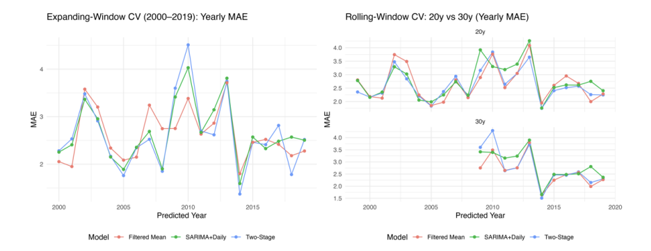
3.2. Cross-validation performance

As shown in Figure 2, this research compared expanding-window CV enlarged training data yearly from 2000 and rolling-window CV with fixed sample sizes of 20 and 30 years for the top three best-performing models. Despite similar overall performance across the three approaches, the Two-Stage Regression and Filtered Mean method outperformed the SARIMA+Typical Day reconstruction model. The fluctuation of MAE is evident in all three subplots for 2010, as the winter of 2009-2010 experienced a climatic anomaly known as the "Big Freeze" [14]. This suggests the models have both strengths and weaknesses.

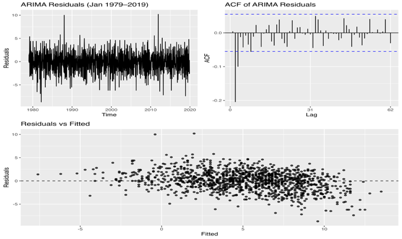
3.3. Residual diagnostics

As shown in Figure 3, residual diagnostics were performed on the ARIMA model fitted to the stacked time series from 1979 to 2020. The residual series resembles a random walk, but the ACF plot of the residuals shows significant autocorrelation when the lag is 1. The Ljung–Box test also rejects the white noise hypothesis (X² = 84.1, df = 20, p < 0.001). These findings suggest that the ARIMA model fails to fully capture time dependence in the data, reflecting that omitting the change between years and concatenating the January data are infeasible.

3.4. Statistical tests

This study adopted the DM-test and the paired t-test to compare the Two-Stage Regression model with the second- and third-best-performing models. The statistics for the absolute error (AE) and squared error (SE) of the DM-test between the Two-Stage Regression and SARIMA+Typical Day Reconstruction methods are -2.45 and -3.50, respectively. Moreover, the p-values for AE and SE are 0.020 and 0.0015, respectively (both less than 0.05), and similar results can be observed in the DM-test between the Two-Stage model and the Filtered Mean method. The experimental values illustrate that the Two-Stage model has a significantly smaller daily prediction error than other top-ranked models. In the paired t-test, the p-value was 0.031 for the experiment comparing Two-Stage Regression with the Filtered Mean method, while a higher value of 0.28 was obtained for the other comparison. The result of the paired t-test suggests that the Two-Stage model has an advantage over the Filtered Mean in the 20-year average. However, its performance is statistically indistinguishable from that of the SARIMA+Typical Day Reconstruction model.

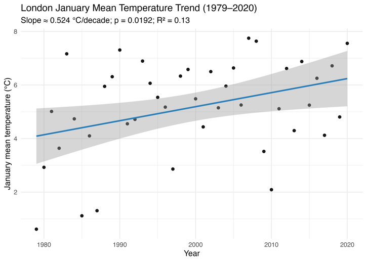
3.5. Climate trend analysis

As shown in Figure 4, OLS regression reveals a positive trend in London monthly average January temperatures between 1979 and 2020, with an estimated slope of approximately 0.52 °C per decade (SE = 0.215, t = 2.44, p < 0.05). Only 13% of the year-to-year variation is explained (R² = 0.13) since temperature exhibits substantial interannual variability [15]. The analysis highlights a persistent rise in winter temperatures, indicating the long-term influence of climate warming.

4. Conclusion

This research evaluated nine various models, including mean-based methods, trend regression models, GAM, and ARIMA family models. The Two-Stage Regression method is the best in terms of MAE and RMSE when predicting January 2020 daily temperatures, and it also has robustness according to the outcomes of CV. Furthermore, in long-term forecasting, the t-test result suggests that it is advisable to consider conducting the SARIMA+Typical Day Reconstruction method. From the residual diagnostics for the ARIMA model, it is evident that the mean daily temperature does not follow a random walk, and ignoring the annual trend is inappropriate. The long-term temperature trend examination in London reaffirms that climate warming has now become an unequivocal reality in recent years, with a significant rate (approximately 0.5 °C per decade).

Methods that capture both within-month fluctuations in January and the yearly warming trend are more likely to yield better predictive performance, as these two features are characteristics of the superior methods (such as SARIMA+Typical Day Reconstruction method and Two-Stage Regression) explored in this study. The findings offer implications for climate adaptation, energy planning, and urban management.

This research provides a unified framework for comparing simple baseline models and statistical methods, but it focuses solely on the mean temperature time series in the London area. Enhancements include applying a machine learning approach to gather more detailed information or using multiple regression with variables such as precipitation and sunshine radiation in the same dataset to improve precision.

References

[1]. M. Kendon, A. Doherty, D. Hollis, E. Carlisle, S. Packman, A. Matthews, S. Jevrejeva, J. Williams, and J. Garforth, "State of the UK Climate 2024, " International Journal of Climatology, vol. 45, no. S1, pp. 1–72, 2025, doi: 10.1002/joc.70010.
[2]. X. Zhang, Y. Li, and J. Wang, "Hybrid ARIMA–machine learning approaches for daily weather prediction, " Atmospheric Research, vol. 290, 106782, 2023, doi: 10.1016/j.atmosres.2023.106782.
[3]. S. Khan, N. Ahmed, and R. Ali, "Comparison of statistical and machine learning models for daily temperature forecasting, " Theoretical and Applied Climatology, vol. 146, no. 1–2, pp. 345–360, 2021, doi: 10.1007/s00704-021-03742-5.
[4]. E. Fwerr, "London Weather Data (1979–2021), " Kaggle, Online dataset.
[5]. R. J. Hyndman and G. Athanasopoulos, Forecasting: Principles and Practice, 3rd ed. OTexts, 2021.
[6]. I. Shah, P. Mubassir, S. Ali, and O. Albalawi, "A functional autoregressive approach for modeling and forecasting short-term air temperature, " Frontiers in Environmental Science, vol. 12, p. 1411237, 2024, doi: 10.3389/fenvs.2024.1411237.
[7]. Q. Xu, Q. Wen, and L. Sun, "Two-Stage Framework for Seasonal Time Series Forecasting, " in Proc. IEEE Int. Conf. on Acoustics, Speech and Signal Processing (ICASSP), pp. 4325–4329, 2021, doi: 10.1109/ICASSP39728.2021.9414118.
[8]. R. J. Hyndman and Y. Khandakar, "Automatic time series forecasting: the forecast package for R, " Journal of Statistical Software, vol. 27, no. 3, pp. 1–22, 2008, doi: 10.18637/jss.v027.i03.
[9]. K. Szostek, "Analysis of the effectiveness of ARIMA, SARIMA, and SVR in seasonal time series forecasting, " Energies, vol. 17, no. 19, p. 4803, 2024, doi: 10.3390/en17194803.
[10]. R. Bassett, X. Cai, L. Chapman, C. Heaviside, and J. Thornes, "The changing intensity of the urban heat island in London, 1990–2019: A comparison of observations and GAM-based trends, " Atmosphere, vol. 12, no. 3, p. 345, 2021, doi: 10.3390/atmos12030345.
[11]. T. Chai and R. R. Draxler, "Root mean square error (RMSE) or mean absolute error (MAE)? – Arguments against avoiding RMSE in the literature, " Geoscientific Model Development, vol. 7, no. 3, pp. 1247–1250, 2014.
[12]. S. Meisenbacher, "Review of automated time series forecasting pipelines, " WIREs Data Mining and Knowledge Discovery, vol. 12, no. 5, e1455, 2022, doi: 10.1002/widm.1455.
[13]. F. X. Diebold and R. S. Mariano, "Comparing predictive accuracy, " Journal of Business & Economic Statistics, vol. 13, no. 3, pp. 253–263, 1995, doi: 10.1080/07350015.1995.10524599.
[14]. R. Cattiaux, R. Vautard, C. Cassou, P. Yiou, V. Masson-Delmotte, and F. Codron, “Winter 2010 in Europe: A cold extreme in a warming climate, ” Geophysical Research Letters, vol. 37, article no. L20704, Oct. 2010, doi: 10.1029/2010GL044613.
[15]. E. Rousi, B. Caldeira, J. Räisänen, and R. J. Greatbatch, “Implications of Winter NAO Flavors on Present and Future European Climate, ” Climate, vol. 8, no. 1, p. 13, Jan. 2020. doi: 10.3390/cli8010013.
Cite this article
Zhang,Y. (2025). Forecasting Daily January Temperatures in London Using Nine Statistical Approaches. Theoretical and Natural Science,132,95-103.
Data availability
The datasets used and/or analyzed during the current study will be available from the authors upon reasonable request.
Disclaimer/Publisher's Note
The statements, opinions and data contained in all publications are solely those of the individual author(s) and contributor(s) and not of EWA Publishing and/or the editor(s). EWA Publishing and/or the editor(s) disclaim responsibility for any injury to people or property resulting from any ideas, methods, instructions or products referred to in the content.
About volume
Volume title: Proceedings of CONF-APMM 2025 Symposium: Simulation and Theory of Differential-Integral Equation in Applied Physics
© 2024 by the author(s). Licensee EWA Publishing, Oxford, UK. This article is an open access article distributed under the terms and
conditions of the Creative Commons Attribution (CC BY) license. Authors who
publish this series agree to the following terms:
1. Authors retain copyright and grant the series right of first publication with the work simultaneously licensed under a Creative Commons
Attribution License that allows others to share the work with an acknowledgment of the work's authorship and initial publication in this
series.
2. Authors are able to enter into separate, additional contractual arrangements for the non-exclusive distribution of the series's published
version of the work (e.g., post it to an institutional repository or publish it in a book), with an acknowledgment of its initial
publication in this series.
3. Authors are permitted and encouraged to post their work online (e.g., in institutional repositories or on their website) prior to and
during the submission process, as it can lead to productive exchanges, as well as earlier and greater citation of published work (See
Open access policy for details).