Interpretable Machine Learning for 100-Yard Freestyle Performance: SHAP-Driven Feature Selection of Lap-Level Stroke, Splits, and Breakout Metrics

1. Introduction

In competitive swimming, for a swimmer to achieve optimal performance in races, technical details in all aspects need to be meticulously executed. The 100-yard freestyle is an event demanding not only power, but also high levels of efficiency and strategic energy distribution. Therefore, it is particularly sensitive to subtle variations in a swimmer's technique across its four 25-yard laps [1]. Modern tracking technologies are transforming the world of competitive swimming, including the way people analyze techniques, by enabling the accurate measurement of various metrics such as stroke rate, cycle count, and breakout distance for each segment of a race. While one might be aware of the importance of these metrics, the complex, non-linear interactions between them make it difficult to objectively determine their relative impact on the final race time [2].

The application of machine learning (ML) in sports analytics offers a powerful solution for modeling such complex relationships. Algorithms like Random Forests [3] and Support Vector Machines [4], both widely adopted ML methods, have proven effective in predicting athletic performance in various domains by capturing intricate patterns within multidimensional data [5]. Recent work has started to apply these techniques to swimming performance prediction [6], demonstrating their potential utility. However, a significant limitation of many powerful ML models is their "black box" nature; they provide accurate predictions without providing intelligible explanations for why a certain outcome is predicted [7]. For sports scientists, and especially for coaches who focus more on practical guidelines than model details, this lack of interpretability hinders the translation of analytical results into actionable training interventions.

This study aims to address this gap by developing a transparent and actionable analytical framework for competitive swimming. We leverage Shapley Additive Explanations (SHAP) [8] on top of classic machine learning methods, a game-theoretic approach that provides consistent and theoretically sound feature importance values, to interpret the output of ML models. This approach allows us to move beyond the confusing numerical output predictions and answer practical questions: Which specific metrics are most predictive of performance in a 100-yard freestyle? How does the importance of a metric change from one lap to another? And, is there a minimal set of key metrics that retains predictive power, which can help simplify performance monitoring for coaches?

The primary objectives of this research are the following: (1) to develop and compare performance among multiple regression and classification models for predicting race times and performance metrics; (2) to employ SHAP values to provide interpretation of the best-performing model, quantifying the impact of each input feature; and (3) to perform feature selection based on this interpretability analysis, evaluating how performance changes when only a subset of features is used.

The contribution of this work is an interpretable ML framework that suggests impacts of technical details on race performance, filling the gap between advanced sports analytics and practical guidelines. The findings provide data-driven evidence to help swimmers prioritize technical focus and training strategies to make informed strategic adjustments to their race to optimize their racing performance.

2. Methods

2.1. Overview of the framework

We developed a comprehensive framework that integrates machine learning prediction with model interpretation to identify key factors for racing performance in competitive swimming. The framework consisted of three steps: 1) data processing and target variable construction, 2) predictive model development, and 3) comparison, and model interpretation with feature importance analysis using SHAP values. These steps allow us to both provide a reasonable prediction to the race outcome and identify the most influential technical factors on these predictions.

2.2. Materials and data

Data were obtained from a publicly available swimming analytics dataset on Kaggle [9], which contains lap-by-lap metrics for 100-yard freestyle performances from the A-Finals swims of the past 10 NCAA championships. The original dataset comprised 268 observations with detailed metrics including “Lap_Number”, “Cycles”, “Avg_Stroke_Rate”, etc.

2.3. Data preprocessing and exploratory data analysis

The framework starts with data preprocessing. The original dataset includes every single swim from the A-finals of the men’s 100-yard freestyle from 2015 to 2024, but without the data in 2020 since the meet is affected by covid-19. There will also be duplicated swimmers in the dataset because one swimmer can qualify for the finals in multiple years and hence, be recorded for multiple times.

We also noticed that 3 race observation data points did not record “breakout_distance”. This missing data was filled in by watching the actual race videos [10] to record the actual breakout distance of the 3 races, adding 3 more complete race observations to the dataset, resulting in a total of 67 valid data samples.

We conducted exploratory data analysis including distribution analysis of race times and K-means clustering to identify natural performance groupings. The results revealed five distinct performance clusters, from which we created a binary classification problem by excluding the middle cluster and thresholding the remaining data at 41.4 seconds to distinguish between faster (class 1) and slower (class 0) performances.

2.4. Problem formulation and feature construction

We formulated the task as two types of prediction problems: (1) a regression problem where the inputs are the 12 lap-specific features and the target output is continuous race time in seconds, and (2) a binary classification problem predicting fast/slow performance categories. We trained multiple popular machine learning models including Linear Regression [11], Random Forest Regressor [12], and k-Nearest Neighbors Regressor for regression [13], and Random Forest Classifier [14], k-Neighbors Classifier [15], and Support Vector Classifier for classification [16].

The target variable was constructed by extracting and summing the 50-yard split times from laps 2 and 4 (y1 and y2) to represent the complete 100-yard race time (y), resulting in 67 complete race observations for final analysis.

We constructed features by organizing three key technical metrics across all four laps: 'Avg_Stroke_Rate', 'Cycles', and 'Breakout Distance (Yards)'. For each swimmer, we constructed these three metrics from all four laps into a single 12-dimensional feature vector using NumPy stacking, creating the final feature matrix X with dimensions (67, 12).

2.5. Model interpretation and feature analysis

We interpreted the impact of features using SHAP (Shapley Additive Explanations) values. This explainable step allowed us to quantify both the magnitude and direction of each feature's influence on predictions, generating global feature importance rankings and individual prediction explanations.

2.6. Training and evaluation

We split the data into training and test sets with 75-25 ratio and fixed random seeds in the algorithms for reproducible results. In addition, to ensure model robustness, we repeated train-test-split and the corresponding training and evaluation 50 times for each model and used the average performance of each model to summarize and compare their performances.

We chose multiple performance evaluation metrics that focus on different aspects of the prediction task. For regression models, we employed R-squared (R²) to measure goodness of fit and Mean Absolute Percentage Error (MAPE) to quantify prediction accuracy. For classification models, we used accuracy and F1-score to provide a balanced assessment of model performance, especially useful when dealing with imbalanced datasets.

To display the results, we generated various plots including performance comparison bar and violin plots, SHAP summary plots for feature importance visualization, and feature selection analysis plots showing the trade-off between model complexity and predictive performance. The analysis was carried out in Python using scikit-learn for machine learning models, SHAP for model interpretation, Seaborn for visualization, with all code executed in a Jupyter notebook environment for reproducible research.

3. Results

We first compared the performances of different machine learning methods on the same task. We then focused on one method, and examined the feature contribution using SHAP (Section 2.5). We also analyzed how the model performs when using a smaller subset of features.

3.1. Data processing

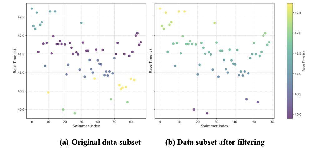
Figure 1. kMeans clustering comparison plot

Initially, the distribution of 50-yard split times showed a wide range (Figure 1, Left). To simplify the problem and focus on the more distinct performance groups, data points from the middle cluster, identified using KMeans clustering with K=5, were removed (Figure 1, Right). The remaining data was then used for subsequent regression and classification analyses. For classification, the continuous race times were converted into a binary target variable based on whether the 100-yard race time was above or below 41.4 seconds, creating "faster" and "slower" categories.

3.2. Regression model comparison

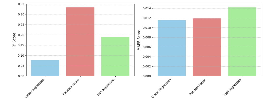
Regression models (Linear Regression, Random Forest, and kNN Regression) were trained to predict the 100-yard race time. A single run evaluation showed varying performance (Figure 2). Random Forest Regression achieved the highest R² score (0.334), while Linear Regression had the lowest MAPE (0.011).

Figure 2. Single run regression model performance

Table 1. Regression model performance with 95% confidence intervals
Method	R² Mean	R² CI	MAPE Mean	MAPE CI
Linear Regression	-0.332	[-0.648, -0.015]	0.011	[0.011, 0.012]
Random Forest	-0.042	[-0.146, 0.061]	0.011	[0.011, 0.013]
KNN Regression	-0.115	[-0.220, -0.011]	0.012	[0.011, 0.012]

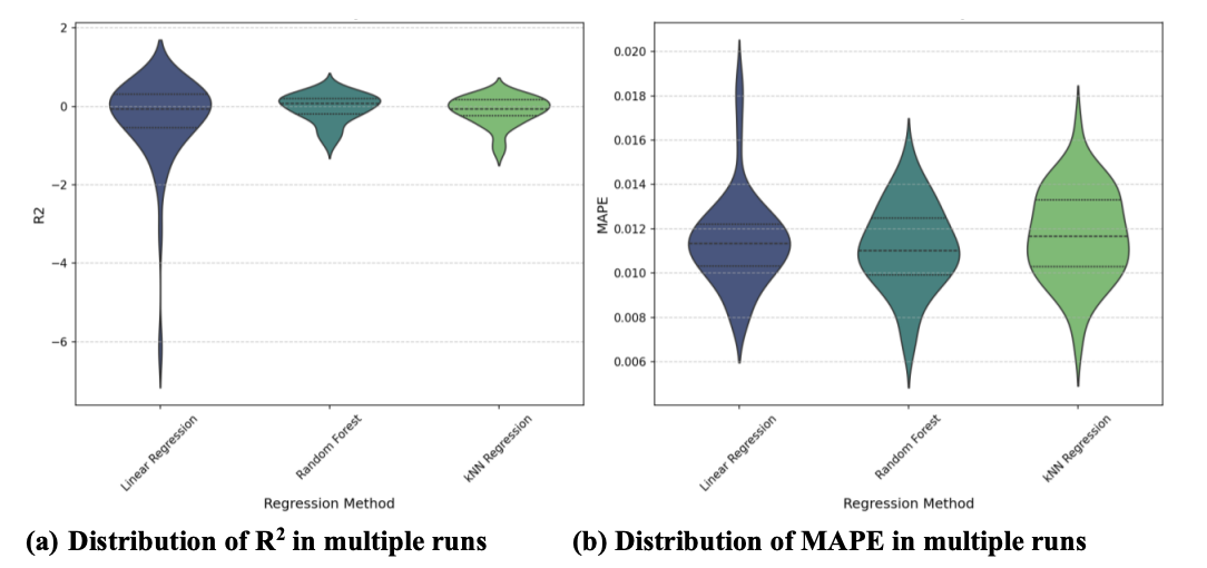
Figure 3. Regression model performance across 50 runs

Recognizing that performance on a single split can be subject to random chance and may not be representative of a model's true predictive capability, a more robust evaluation was conducted across 50 different random train-test splits. By employing multiple splits and calculating performance metrics for each, we can assess the variability of the models' performance and derive more reliable estimates through confidence intervals. The results from these multiple runs, including 95% confidence intervals, are presented in Table 1 and visualized using violin plots in Figure 3.

The evaluation across 50 runs revealed that the regression task is challenging with the current dataset and features. The mean R² scores for all models were low, with confidence intervals frequently overlapping zero or extending into negative values (Table 1, Figure 3). A negative R² indicates that the model performs worse than simply predicting the mean of the target variable. This collectively suggests that a substantial portion of the variance in 100-yard race time remains unexplained by the selected features when using these regression models. The violin plots (Figure 3) further illustrate the variability in R² performance across different splits for all models, highlighting their sensitivity to the specific data used for training and testing. Despite the low R² values, the mean MAPE scores were consistently low and clustered tightly around 0.011-0.012 for all models, with narrow confidence intervals. This suggests that while the models struggle to capture the underlying patterns and explain variance (low R²), the average prediction error compared to the actual race time is relatively small. Among the models, Random Forest Regression showed the highest mean R² (-0.042), although its confidence interval largely overlapped with those of Linear Regression (-0.332 [-0.648, -0.015]) and kNN Regression (-0.115 [-0.220, -0.011]), indicating no statistically significant difference in mean R² performance at the 95% confidence level. Similarly, MAPE values were comparable across models.

3.3. Classification model comparison

In addition to regression models, the classification models were trained to predict a binary performance category, either “faster” or “slower”, based on whether a swimmer’s 100-yard race time was above or below a predefined boundary. Three classification models were evaluated and compared: Random Forest classifier, kNN Classifier, and Support Vector Classifier (SVC). Model Performance was evaluated using Accuracy, measuring the overall proportion of correct classifications, and F1 Score, providing a balanced assessment of model performance.

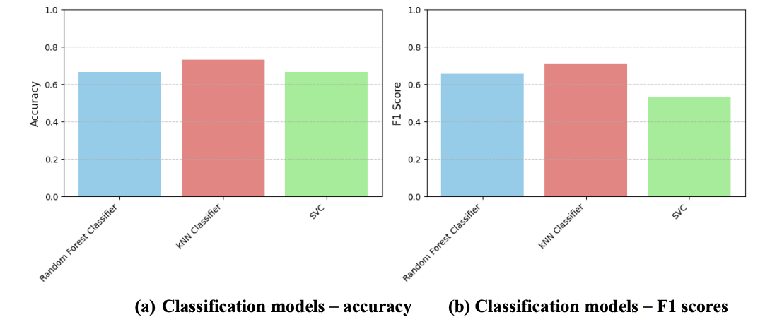
A single run evaluation on a fixed train-test split (Figure 4) showed that all models performed above 50% accuracy for a balanced binary classification. The kNN Classifier achieved the highest Accuracy (0.733), closely followed by Random Forest Classifier (0.667) and SVC (0.667). In terms of F1 score, kNN Classifier (0.712) performed above Random Forest Classifier (0.656) and SVC (0.533) as well.

Figure 4. Single run classification model performance

Table 2. Classification model performance with 95% confidence intervals
Method	Accuracy Mean	Accuracy CI	F1 Score Mean	F1 Score CI
Random Forest	0.673	[0.612, 0.735]	0.668	[0.616, 0.719]
KNN Classifier	0.727	[0.635, 0.818]	0.717	[0.628, 0.807]
SVC	0.673	[0.658, 0.688]	0.555	[0.521, 0.589]

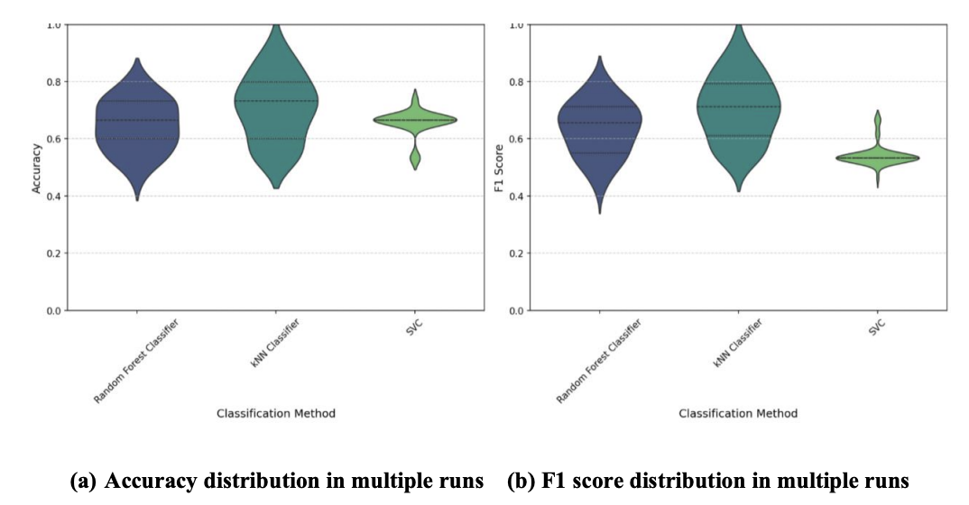
Figure 5. Classification model performance across 50 runs

To obtain a more robust understanding of classification performance and its variability, each classification model was evaluated across 50 random train-test splits, employing stratified sampling to ensure the proportion of "faster" and "slower" swimmers was maintained in each split. Table 2 summarizes the mean Accuracy and F1 Scores along with their 95% confidence intervals, while Figure 5 provides a visual representation of the performance distributions using violin plots.

Across 50 runs, the kNN Classifier demonstrated advanced performance compared to the other classification models. It has the highest mean Accuracy (0.727) with a 95% confidence interval of [0.635, 0.818], and the highest mean F1 Score (0.717) with a 95% confidence interval of [0.628, 0.807]. The confidence intervals for kNN Classifier were also in a tighter range than the confidence intervals of Random Forest Classifier, suggesting less variability in its performance across different data splits. SVC showed a comparable mean Accuracy (0.673) to Random Forest Classifier but a notably lower mean F1 Score (0.555), indicating potential issues of precision despite high overall accuracy. These results suggest that the kNN Classifier is the most effective model among those tested for distinguishing between "faster" and "slower" swimmers based on the provided features.

3.4. Feature importance analysis using SHAP

Among the several models evaluated, the Random Forest Regression Model was not only on the high-performance side, but also was specifically selected for being capable to perform deep feature interpretability analysis using SHAP (Shapley Additive exPlanations). This decision was driven by SHAP’s robust framework of explaining predictions based on tree-based models, providing a detailed understanding of how individual features contribute to the model’s output. Although other models demonstrated competitive performance in prediction, the Random Forest’s compatibility with SHAP allowed for a more nuanced exploration of feature contributions on race time.

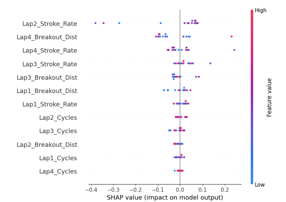
Figure 6. SHAP summary plot: Feature impact on race time prediction

To gain insights into which features most influence the predicted race time by the Random Forest Regression model, SHAP values were calculated. SHAP values quantify the contribution of each feature to the difference between a prediction and the average prediction across the dataset. The SHAP summary plot (Figure 6) provides a global view of feature importance and the distribution of SHAP values for each feature across the test dataset.

Table 3. Top 5 most important features and their influence
Feature	SHAP Importance	Influence
Lap2_Stroke_Rate	0.113809	Decrease Race Time
Lap4_Breakout_Dist	0.080193	Mixed Impact
Lap4_Stroke_Rate	0.044282	Increase Race Time
Lap3_Stroke_Rate	0.031122	Increase Race Time
Lap4_Breakout_Dist	0.030486	Mixed Impact

The analysis revealed that 'Lap2_Stroke_Rate' was the most influential feature, with a mean absolute SHAP value of 0.114. Higher values of 'Lap2_Stroke_Rate' were generally associated with lower predicted race times (i.e., faster swims), indicated by a negative correlation between the feature value and its SHAP value. Other highly influential features included 'Lap4_Breakout_Dist' and 'Lap4_Stroke_Rate'. 'Lap4_Breakout_Dist' showed a mixed impact, while higher 'Lap4_Stroke_Rate' values tended to increase predicted race times (i.e., slower swims). Features related to Cycles generally had lower importance compared to Stroke Rate and Breakout Distance. This feature importance analysis highlights the critical role of stroke rate and breakout distance, particularly in later laps, in determining predicted race time.

3.5. Feature selection and model efficiency

Given the insights from the feature importance analysis, the potential for model simplification and improved efficiency through feature selection was explored. A reduced feature set consisting of the top 3 most important features identified by SHAP ('Lap2_Stroke_Rate', 'Lap4_Breakout_Dist', and 'Lap4_Stroke_Rate' based on the latest calculation) was used to train a new Random Forest Regression model. The performance of this model with the reduced feature set was then compared to the performance of the model trained on the full set of 12 features using R² and MAPE metrics, as shown in figure 7.

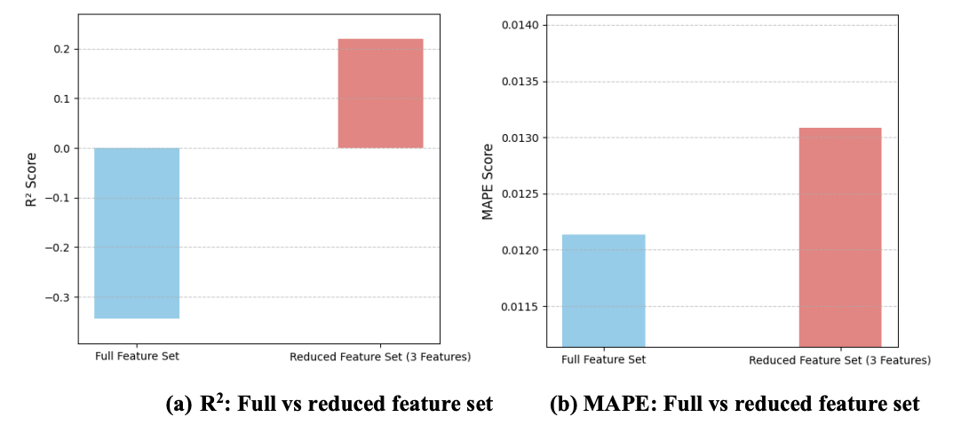
Figure 7. Full vs reduced feature set comparison

Further analysis explored the impact of feature selection on the Random Forest Regression model's performance, focusing on a reduced set of the top 3 features identified through SHAP analysis (Figure 7 and Figure 8). The comparison revealed a trade-off between model complexity and predictive metrics. While the R² score, which measures the proportion of variance, was slightly lower with the 3-feature set compared to the full 12-feature set in this single evaluation, the Mean Absolute Percentage Error (MAPE) remained notably similar. This indicates that a substantial reduction in the number of input features can be achieved at the cost of only a minimal decrease in the average percentage accuracy of predictions. This outcome is significant from an efficiency perspective, suggesting that a significantly simpler model, requiring fewer data inputs and potentially less computational resources, can achieve comparable predictive accuracy in terms of variability, making it a more effective option for swim coaches and athletes who want to focus on particular techniques.

4. Discussion

The research in this work explored the application of machine learning to predict and classify swimming performance from kinematic and physiological data. The multiple linear regression to predict continuous 100-yard swim times had no significant predictive ability with the current feature set and amount of data, indicated by low and fluctuating R² values. This would suggest that the features selected, while perhaps related to performance, fail to represent highly involved determinants of precise race times in this model framework. In contrast, the class model, designed to distinguish the swimmers into "faster" or "slower" classes, produced more promising results, particularly in the instance of the kNN Classifier. This suggests that distinction between general levels of performance is more with this data than with the prediction of precise times. The SHAP-based feature importance analysis provided valuable insights into the model's decision-making, identifying the key contributions of stroke rate and breakout distance, especially in later laps. For example, the negative contribution of 'Lap2_Stroke_Rate' to predicted race time implies that an increasing stroke rate towards the start of the race is associated with enhanced performance outcomes.

Direct comparison to the literature is not easy due to the specificity of the dataset and features, but the implications regarding the applicability of stroke rate and breakout distance are in line with general biomechanics principles in swimming. Efficient stroke technique and high breakouts at the high level of swimming occur as attempts to minimize drag and maximize propulsion. The challenge to get high R² for continuous performance prediction is not uncommon in sport science, where human variability and the biological system nature can make precise prediction challenging. Success with classification over regression agrees with expectations that it is simpler to discriminate between clearly different groups than to predict continuous values.

There are also several limitations. The dataset is of medium size, which should have resulted in the wide variation of the performance of the regression models and large confidence intervals. Having a larger dataset would be possible with more statistical significance. The binary classification goal was defined by a single threshold and may not capture the nuances of performance categorization; alternative clustering or multi-class classification procedures might be worth exploring. Data used for analysis were limited to a specific set of features; inclusion of additional data streams, such as other swim phases or physiological data, could enhance predictive accuracy. Finally, the models were evaluated using typical metrics; investigation into the application of alternative evaluation metrics distinct to swimming performance might be enlightening.

The findings have several implications for coaching and swimming analysis. The performance of the classification models suggests the potential to utilize machine learning to objectively categorize swimmers by performance level, which may have application for talent identification or individualized training regimens. The analysis of feature importance provides empirical data regarding the most significant technical features (e.g., stroke rate and breakout distance) in determining performance according to the models, which guides coaches on where to focus training efforts. The outputs of feature selection demonstrate that with a reduced set of meaningful features, decent prediction performance is still attainable, showing potential in developing more cost-efficient and less data-hungry performance analysis software.

5. Conclusion

In conclusion, this study successfully applied machine learning techniques to analyze swimming performance data, demonstrating the feasibility of classifying swimmers into performance groups despite the challenges in precisely predicting continuous race times with the current datasets.

The primary findings highlight the kNN Classifier as the most effective model for binary performance classification and underscore the significant influence of features such as stroke rate and breakout distance on predicted race time, as revealed by SHAP analysis.

This project contributes to the application of interpretable machine learning in sports science by providing a framework for analyzing swimming data and identifying key performance indicators. The demonstration of effective feature reduction while maintaining comparable predictive accuracy (in terms of MAPE) also contributes to the development of more efficient analytical tools in this domain.

Future research should focus on acquiring larger and more diverse datasets to improve model robustness and potentially enhance regression performance. Exploring advanced feature engineering techniques and incorporating a wider range of physiological and biomechanical data could provide deeper insights. Investigating multi-class classification or clustering approaches for performance categorization and applying time-series models to capture the dynamic nature of swimming would also be valuable next steps.

References

[1]. Rozi, G., Mavromatis, G., Toubekis, A., & Ozen, S. (2018, January 1). Relationship between force parameters and performance in 100 m front crawl swimming. Sport Science, 11(1), 57–60.https: //www.researchgate.net/publication/330344100_Relationship_between_force_parameters_and_performance_in_100m_front_crawl_swimming

[2]. Figueiredo, P., Zamparo, P., Sousa, A., Vilas-Boas, J. P., & Fernandes, R. J. (2013). Interplay of biomechanical, energetic, coordinative, and muscular factors in a 200 m front crawl swim. BioMed Research International, 897232. https: //doi.org/10.1155/2013/897232

[3]. Breiman, L. (2001, October). Random Forests. Machine Learning, 45(1), 5–32. https: //doi.org/10.1023/A: 1010933404324

[4]. Cortes, C., & Vapnik, V. (1995, September). Support-vector networks. Machine Learning, 20(3), 273–297. https: //doi.org/10.1007/BF00994018

[5]. Bunker, R. P., & Thabtah, F. (2019, January). A machine learning framework for sport result prediction. Applied Computing and Informatics, 15(1), 27–33. https: //doi.org/10.1016/j.aci.2017.09.005

[6]. Xie, J., Wang, J., Zhang, Z., & Zhang, Y. (2016, October). Machine learning of swimming data via wisdom of crowd and regression analysis. Mathematical Biosciences and Engineering, 13(6), 9–19. https: //doi.org/10.3934/mbe.2017031

[7]. Rudin, C. (2019, May). Stop explaining black box machine learning models for high-stakes decisions and use interpretable models instead. Nature Machine Intelligence, 1(5), 206–215. https: //doi.org/10.1038/s42256-019-0048-x

[8]. Lundberg, S. M., & Lee, S.-I. (2017, November 24). A unified approach to interpreting model predictions. Proceedings of NIPS (arXiv: 1705.07874). https: //arxiv.org/abs/1705.07874

[9]. justinr111. (2024). NCAA 100 Freestyle 2015–2024 (Kaggle dataset). Kaggle. https: //www.kaggle.com/datasets/justinr111/ncaa-100-freestyle-2015-2024

[10]. NCAA Men’s Swimming. (2025, March 30). 10 Years of the Men’s 100 Freestyle – NCAA Edition (2014-2024) [Video]. YouTube. https: //youtu.be/YpVjiKIgS6g

[11]. Scikit-learn developers. (2023). LinearRegression. scikit-learn 1.7.2 documentation. https: //scikit-learn.org/stable/modules/generated/sklearn.linear_model.LinearRegression.html

[12]. Scikit-learn developers. (2023). RandomForestRegressor. scikit-learn 1.7.2 documentation. https: //scikit-learn.org/stable/modules/generated/sklearn.ensemble.RandomForestRegressor.html

[13]. Scikit-learn developers. (2023). KNeighborsRegressor. scikit-learn 1.7.2 documentation. https: //scikit-learn.org/stable/modules/generated/sklearn.neighbors.KNeighborsRegressor.html

[14]. Scikit-learn developers. (2023). RandomForestClassifier. scikit-learn 1.7.2 documentation. https: //scikit-learn.org/stable/modules/generated/sklearn.ensemble.RandomForestClassifier.html

[15]. Scikit-learn developers. (2023). KNeighborsClassifier. scikit-learn 1.7.2 documentation. https: //scikit-learn.org/stable/modules/generated/sklearn.neighbors.KNeighborsClassifier.html

[16]. Scikit-learn developers. (2023). SVC. scikit-learn 1.7.2 documentation. https: //scikit-learn.org/stable/modules/generated/sklearn.svm.SVC.html

Cite this article

Wang,Z. (2025). Interpretable Machine Learning for 100-Yard Freestyle Performance: SHAP-Driven Feature Selection of Lap-Level Stroke, Splits, and Breakout Metrics. Theoretical and Natural Science,151,1-11.

Data availability

The datasets used and/or analyzed during the current study will be available from the authors upon reasonable request.

Disclaimer/Publisher's Note

The statements, opinions and data contained in all publications are solely those of the individual author(s) and contributor(s) and not of EWA Publishing and/or the editor(s). EWA Publishing and/or the editor(s) disclaim responsibility for any injury to people or property resulting from any ideas, methods, instructions or products referred to in the content.

About volume

Volume title: Proceedings of CONF-CIAP 2026 Symposium: Applied Mathematics and Statistics

ISBN：978-1-80590-559-2(Print) / 978-1-80590-560-8(Online)

Editor：Marwan Omar

Conference website: https://www.confciap.org/chicago.html

Conference date: 27 January 2026

Series: Theoretical and Natural Science

Volume number: Vol.151

ISSN：2753-8818(Print) / 2753-8826(Online)

© 2024 by the author(s). Licensee EWA Publishing, Oxford, UK. This article is an open access article distributed under the terms and conditions of the Creative Commons Attribution (CC BY) license. Authors who publish this series agree to the following terms:
1. Authors retain copyright and grant the series right of first publication with the work simultaneously licensed under a Creative Commons Attribution License that allows others to share the work with an acknowledgment of the work's authorship and initial publication in this series.
2. Authors are able to enter into separate, additional contractual arrangements for the non-exclusive distribution of the series's published version of the work (e.g., post it to an institutional repository or publish it in a book), with an acknowledgment of its initial publication in this series.
3. Authors are permitted and encouraged to post their work online (e.g., in institutional repositories or on their website) prior to and during the submission process, as it can lead to productive exchanges, as well as earlier and greater citation of published work (See Open access policy for details).