1. Introduction

In engineering and science, the need for modeling and simulations of airflow over objects, such as airfoils, buildings, aircraft, and cars, is of utmost importance. Before the advent of computers capable of performing such complex tasks, calculations had to be done mostly by hand, which could only handle simple problems with reduced accuracy. With the introduction of more powerful computers, computational fluid dynamics (CFD) could be used to simulate fluid dynamics, thus allowing engineers to model the flow of air and its interactions with objects quickly. CFD adopts computer programs to solve partial differential equations (PDEs), which describe the mass, momentum, and energy conservation of the flow. There are three advantages of using CFD for engineering designs: First, it is faster than other design methods, allowing multiple designs to be simulated within a short period of time. Second, compared with the previous methods of design by hand, the CFD approach is more accurate with the high computational power of modern computers. Finally, the cost of design by using CFD is much less than the use of an experimental design, for which a wind tunnel test is normally needed.

In this work, we apply CFD to the simulation of fluid dynamics around an airfoil. The CFD calculations have been performed using Python, including packages of Numpy, Matplotlib, and so on for different purposes. The governing equation describing the fluid motion has been used to achieve the CFD simulation of the airfoil. Compared with the traditional CFD methods, the current work adopts the small disturbance equation for modeling the flow over the airfoil, which could provide a much faster design method for the fluid dynamics over airfoils. We also visualized the flow field over the airfoil and analyzed the different parameters describing the airfoil shape. Finally, we conclude with the results and discussion.

2. Background

In this section, the development of CFD methods will be reviewed to further demonstrate the capability of CFD for different problems in engineering and science. Then, the specific problem of designing the airfoil by using CFD will be further discussed, which is the focus of the current work. Furthermore, we demonstrate that the CFD approach can be useful for the fast and accurate design of airfoils as well as many other fluid dynamics problems.

2.1. Computational Fluid Dynamics

In CFD calculations, we use computers to solve the governing equations of fluid dynamics, which are normally PDEs. First, the conservation of mass needs to be considered, which is also called the continuity equation. Then, the conservation of momentum also needs to be considered. This governing equation essentially is Newton’s second law of mechanics:

\( F=ma\ \ \ (1) \)

where \( F \) is the force, \( m \) is the mass, and \( a \) is the acceleration. In addition to mass and momentum conservation, we need to further consider energy conservation.

In fluid mechanics, Newton’s second law can be expressed as the Navier-Stokes equation, which governs the motion of fluids around the airfoil:

\( ρ\frac{Du}{Dt}=-∇p+∇\cdot τ+ρg\ \ \ (2) \)

The Navier-Stokes equation can be rearranged and reformatted into the Small Disturbance equation, which will be touched on later in the paper and forms the crux of this processing model.

However, computers cannot handle continuous functions. Therefore, we need to initially discretize these equations to solve them using computers. In mapping out space, we can use a discretized mesh for describing the data. For example, the \( x \) -axis can be described by the array [ \( {x_{0}}, {x_{1}}, {x_{2}}…{x_{N}} \) ], which is commonly selected with equal spacing such that:

\( {x_{1}}-{x_{0}}={x_{2}}-{x_{1}}=…={x_{N}}-{x_{N-1}}=Δx\ \ \ (3) \)

Then, the equations can be solved on these meshes by using proper numerical methods.

Many different numerical methods have been developed to deal with different types of fluid dynamics problems [1, 2]. Furthermore, when modeling fluid dynamics using CFD, the more general the method, the less general the boundary geometry, which describes the shapes of the objects it can deal with [3]. Also, it is important to verify and validate the results from CFD, which can be done by the quantification of uncertainty [4]. Different methods have been developed for CFD, for example, the finite volume method [5]. CFD has been successfully applied to various applications [6][7][8].

CFD however requires from the computer running the program sufficient memory, efficient coding, and applicability to different situations. Without paying attention to these factors, the CFD simulation may run slower and less efficiently than needed, costing engineers and companies priceless time and energy. As it stands, there are multiple types of programs that execute CFD, each of which has its advantages and disadvantages. Thus, it is important to adopt the proper algorithms of CFD for specific tasks. In the current project, we will investigate the specific problem of airfoil design with CFD, for which the development of CFD-based airfoil design will be discussed in the next section.

2.2. Airfoil Design with CFD

An important object used in engineering industries and other such industries that use CFD analysis is the airfoil. Figure 1 gives an example of the CFD simulation results for the pressure field over an airfoil. The airfoil is an integral part of aircraft, wind turbines, and even structures like bridges or buildings. Because of the need to understand how an airfoil interacts with air to generate lift, reduce drag, and increase stability, CFD simulations are often used to study and analyze airfoil characteristics. In this fashion, the airfoil best suited for a certain application can be ascertained with better certainty than by manual calculation. In addition, the experimental test of airfoils can be very expensive. Hence, CFD designs can be a fast and accurate way to solve airfoil design problems.

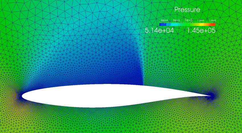
Figure 1. Airfoil pressure field from CFD calculation.

Airfoil design can be studied and perfected by analyzing CFD simulation results. For example, three families of airfoils (the NACA series, FX series, and S series) have been investigated by using CFD [9]. Variable-fidelity optimization algorithms have been applied for the CFD-based optimization of the airfoil shape [10]. The transition model for general CFD codes has been used for predicting the performance of 2D airfoils [11]. It is important to acknowledge that CFD can be used for models with multiple dimensions, like with a 3D model or a 2D model, which usually requires less processing and time [12]. The use of CFD for studying airfoil design is not limited to merely individual models of airfoils, but also to applications that include airfoil characteristics. This can be seen in CFD simulations of wind turbines, which incorporate airfoils while the angle of fluid direction is different from simulations with individual airfoils [13-15]. This flexibility in CFD simulations when analyzing airfoils allows industries and this paper to determine the quality of an airfoil more efficiently. Boundary conditions are also necessary in CFD design, as to not include the space within the airfoil model in the calculations of airflow characteristics. On the surface of the airfoil, the normal force is redirected perpendicularly from the surface, and airflow is redirected away at differing angles depending on the angle of attack. The inlet where the air and airflow are located inside has boundaries as well, which are frictionless. This means air cannot pass through the walls of the inlet but can travel at a uniform velocity within it, before reaching the airfoil obstruction.

3. Design Approach

For the design approach, we adopt Python programming to solve the simplified governing equations of fluid dynamics. Subsequently, airfoils with several different shapes can be modeled. Then, based on these selected airfoil shapes, a new airfoil with better performance can be obtained from the redesign process. The design approach of using CFD for the fluid dynamics of airfoils has been demonstrated in Fig. 2.

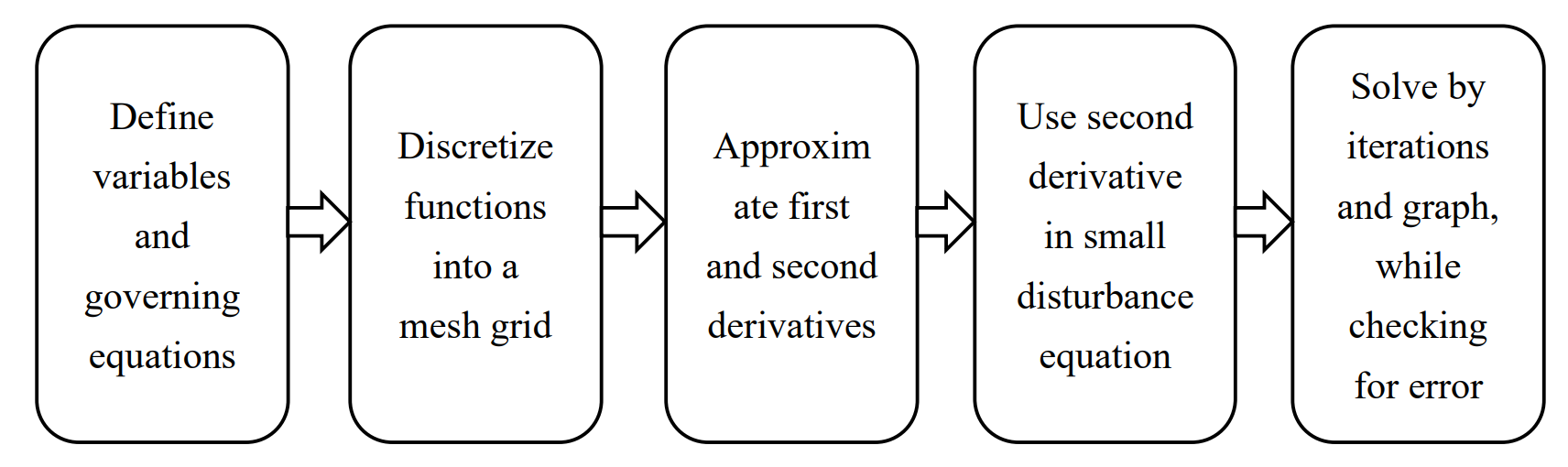
Figure 2. Flowchart for the CFD design approach.

The implementation of the CFD calculations has been realized by using Python, with the two packages of Numpy and Matplotlib. The reason for choosing Python as the programming language is that it is easy to program and provides us with the mathematical functions needed for CFD calculations. The Numpy provides the functions of mathematical calculations, especially these operations on arrays; and the Matplotlib helps us to plot the data in different types of figures.

For solving the governing equations of fluid dynamics, computers can only deal with discrete functions rather than continuous functions. Then, when solving the PDEs with computer algorithms, we need to find the approximations of the derivatives based on the discrete values. For a given function:

\( y=f(x)\ \ \ (4) \)

We need to discretize it into the values on the mesh grids:

\( {x_{0}}=0, {x_{1}}=Δx, {x_{2}}=2Δx,…,{x_{N}}=NΔx\ \ \ (5) \)

for which \( N \) is the number of grid cells and \( Δx \) is the grid size. Then, the \( y \) values on the grids are:

\( {y_{0}}=f({x_{0}}), {y_{1}}=f({x_{1}}), {y_{2}}=f({x_{2}}),…, {y_{N}}=f({x_{N}})\ \ \ (6) \)

In this way, we have transferred the original continuous function into a discrete set of grid values. In solving the PDEs, we also need to approximate the derivatives based on these discrete values. For the first-order derivative, \( \frac{dy}{dx}=\frac{df(x)}{dx} \) at the grid of index \( i \) , we can approximate it as:

\( {(\frac{dy}{dx})_{i}}≈\frac{{y_{i}}-{y_{i-1}}}{{x_{i}}-{x_{i-1}}}=\frac{{y_{i}}-{y_{i-1}}}{Δx}\ \ \ (7) \)

Alternatively, we can express it as,

\( {(\frac{dy}{dx})_{i}}≈\frac{{y_{i+1}}-{y_{i}}}{Δx} \)

\( {(\frac{dy}{dx})_{i}}≈\frac{{y_{i+1}}-{y_{i-1}}}{2Δx}\ \ \ (8) \)

For a PDE describing the wave propagation, the direction of the wave will determine which method to use for the derivative approximation. For the second-order derivative, \( \frac{{d^{2}}y}{d{x^{2}}} \) can be approximated as:

\( {(\frac{{d^{2}}y}{d{x^{2}}})_{i}}≈\frac{{y_{i+1}}-2{y_{i}}+{y_{i-1}}}{Δ{x^{2}}}\ \ \ (9) \)

which is called the central difference method. In most of the governing equations of fluid dynamics, the highest order of the derivative is the second order. Thus, we can now express the governing equations of fluid dynamics by using these approximations on the mesh grid.

The simplified model of the small disturbance equation (SDE) will be used for modeling the flow over the airfoil. The SDE can be expressed as:

\( (1-{Ma^{2}}){ϕ_{xx}}+{ϕ_{yy}}=0\ \ \ (10) \)

where \( Ma \) is the Mach number and \( ϕ \) is the velocity potential. The Mach number is the ratio of the local flow velocity to the local speed of sound. This definition can be expressed as:

\( Ma=\frac{u}{c}\ \ \ (11) \)

where \( u \) is the local flow velocity and \( c \) is the local speed of sound. Therefore, with a greater local flow velocity comes a greater Mach number. The faster the airfoil is traveling, and the greater the Mach number, the more air it is displacing and disturbing. This provides a challenge to the stability of the airfoil and modifies the air pressure and density around the airfoil. Thus, it is important to use the SDE to help model the flow over the airfoil and find its best capabilities under the right conditions. For the current design project, we adopt the SDE, which is the simplified governing equation of fluid dynamics. As such, the computational cost of the CFD can be relatively low compared with other governing equations. In this way, we can do the design process for multiple different airfoil shapes and obtain the optimal design among them.

For the computation of this equation, we can use the previous formula for the second-order derivatives:

\( {{({ϕ_{xx}})_{i,j}}=(\frac{{d^{2}}ϕ}{d{x^{2}}})_{i,j}}≈\frac{{ϕ_{i+1,j}}-2{ϕ_{i,j}}+{ϕ_{i-1,j}}}{Δ{x^{2}}} \)

\( {{({ϕ_{yy}})_{i,j}}=(\frac{{d^{2}}ϕ}{d{y^{2}}})_{i,j}}≈\frac{{ϕ_{i,j+1}}-2{ϕ_{i,j}}+{ϕ_{i,j-1}}}{Δ{y^{2}}}\ \ \ (12) \)

Further, we select \( Δx=Δy=h \) . The equation at \( Ma=0 \) becomes:

\( \frac{{ϕ_{i+1,j}}-2{ϕ_{i,j}}+{ϕ_{i-1,j}}}{Δ{x^{2}}}+\frac{{ϕ_{i,j+1}}-2{ϕ_{i,j}}+{ϕ_{i,j-1}}}{Δ{y^{2}}}=0 \)

\( \frac{{ϕ_{i+1,j}}+{ϕ_{i-1,j}}+{ϕ_{i, j+1}}+{ϕ_{i,j-1}}}{4}-{ϕ_{i,j}}=0\ \ \ (13) \)

\( Ma \) is set to 0 because the airflow velocities being used in this work are substantially low, making the value negligible in calculations and approach 0. Then for this simplified equation, we can solve it by iterations. The Python code for solving this equation is listed as follows:

for i in range(1, newphi.shape[0] - 1):

for j in range(1, newphi.shape[1] - 1):

A_1 = 1

A_2 = 1

B_1 = 1

B_2 = 1

C = 4

dp = - newphi[i, j] + (B_1 * newphi[i, j+1] + B_2 * newphi[i, j-1] +

A_1 * newphi[i+1, j] + A_2 * newphi[i-1, j])/C

newphi[i, j] += dp

4. Results and Discussion

We are going to model the flow over the airfoil by using CFD. The simulations have been conducted in a two-dimensional space with x and y directions. The initial flow velocity is in the x direction, and the orientation of the airfoil is along the x direction. Then, the y direction is vertical to the x direction. By analyzing the velocity fields in both the x and y direction, we can learn how the airfoil affects the fluid dynamics near it. Importantly, the variables used in the figures are dimensionless. For example, the x-axis represents the physical length divided by the specific characteristic length in the problem. This allows for the cancellation of units and improved flexibility of the model to solve problems with different characteristic lengths. (e.g., different airfoil lengths) Next, we are going to discuss several aspects of this issue.

4.1. Airfoil Flow Characteristics

Figure 3. The x-direction velocity distribution of the airfoil.

First, we choose the shape of the airfoil as a sin function. The results of the flow velocity in the x direction have been demonstrated in Fig. 3. It shows that in the front and back of the airfoil, the flow velocity in the x direction is lower than the incoming velocity. This is because when the flow hits the front of the airfoil, the flow field will diverge to the y direction, and hence the velocity in the x direction will be decreased. Differently, in the middle of the airfoil, due to the compression of the flow field near the center of the airfoil, the flow in the x direction will be accelerated and reach a higher velocity compared with the incoming velocity.

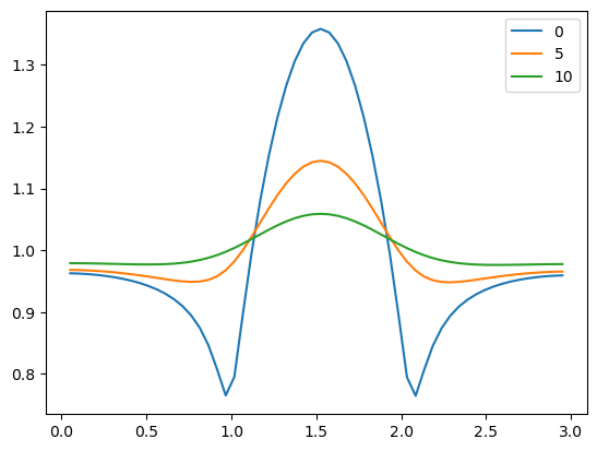
Figure 4. The x-direction velocity distributions at different y locations.

In Fig. 4, we demonstrate the x-direction velocity at different y locations. If the location in the y direction moves away from the surface of the airfoil, the modification of the flow field is less. This is because when we move away from the airfoil surface, the flow is less affected by the airfoil. The closer to the center of the airfoil in the x-direction, however, the greater the x-direction velocity. This can be seen in the large parabolic curve at the 1.5 x-location, which decreases and rebounds near the endpoints of the airfoil.

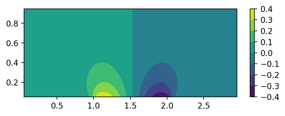
Figure 5. The y-direction velocity distribution of the airfoil.

The mapped velocity distribution here is like Fig. 3, but instead of the x-direction it is the y-direction that is being mapped in Fig. 5. The two halves of the distribution shown appear to be mirror images of each other. There is a drastic positive increase in y-direction velocity at the front of the airfoil, which flips after crossing a point along the airfoil into a decreasing negative velocity. This occurs because the front of the airfoil mainly redirects air upwards quickly, which travels along the airfoil gradually downwards until it reaches the end of the airfoil. At the back of the airfoil, the air is sent drastically downwards, thus giving it a negative velocity.

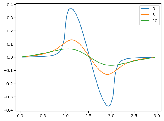
Figure 6. The y-direction velocity distributions at different y-locations.

Next, we look at the y-direction velocity distribution along the x-axis at different y-locations. The y-direction velocity distributions in Fig. 6 show the velocities decreasing in magnitude as the distance from the airfoil increases, in the same fashion as the x-direction velocity distributions. This happens because, with a greater distance from the airfoil, less air is affected by the airfoil being an obstacle. Therefore, the y-direction velocities decrease greatly even with a small distance away from the airfoil location. However, the velocities follow the same general trend of increasing positively at the front of the airfoil and then decreasing into negative velocities at the end of the airfoil, showing how the airflow is still eventually affected. There is also a convergence point along the airfoil where no matter the y-location, the y-direction velocity is 0, corresponding to completely linear horizontal flow.

4.2. Influence of the Airfoil Shapes

In this section, we will examine the influence of the airfoil shape by simulating the flow fields over the airfoils with different shapes. In the previous section, the airfoil shape has been assumed as a sin function:

\( f(x)=sin{[π(x-1)]}\ \ \ (14) \)

for the x direction range from 1 to 2. It should be noted that the shape function goes to zero at both \( x=1 \) and \( x=2 \) , which is because the shape function must be a closed curve at these two locations.

In addition to the sin function shape, we have also tested the airfoil shapes of three other functions, which are the parabolic function, symmetric triangle function, and asymmetric triangle function. For the parabolic function, we have used the form of shape function:

\( f(x)=(x-1)(2-x)\ \ \ (15) \)

which also has the value of zero at both \( x=1 \) and \( x=2 \) . The triangle shapes have two forms. One is the symmetric form:

\( f(x)=x-1 when 1 \lt x \lt 1.5 \)

\( f(x)=2-x when 1.5 \lt x \lt 2\ \ \ (16) \)

This function is continuous at the point of \( x=1.5 \) . However, the derivative of this function is not continuous at \( x=1.5 \) . Another triangle shape that has been used is:

\( f(x)=x-1 when 1 \lt x \lt 1.2 \)

\( f(x)=\frac{2-x}{4}when 1.2 \lt x \lt 2\ \ \ (17) \)

This function is also continuous at the point of \( x=1.2 \) . However, the derivative is not continuous at \( x=1.2 \) . Furthermore, to control the shape of the airfoil, a parameter \( β \) has been multiplied by the shape function.

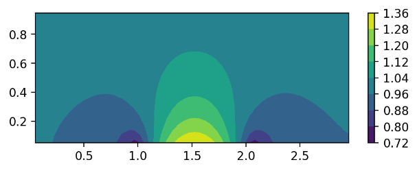
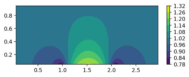
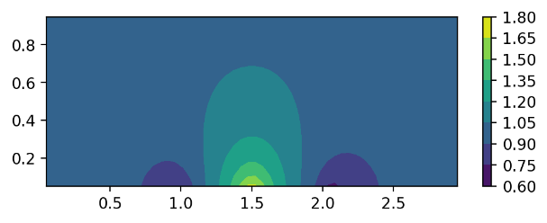
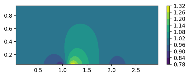
Figure 7. The x-direction velocity distributions of different airfoil shapes. (a) sin function; (b) parabolic function; (c) symmetric triangle function; (d) non-symmetric triangle function.

The CFD simulations of these four different airfoil shapes have been performed. Now we demonstrate the results from these four different airfoil shapes and discuss the reasons why they are different. Figure 7 shows the x-direction velocity distribution of the four different shapes. The top left subfigure is the result of the sin function; the top right subfigure is the result of the parabolic function; the left bottom subfigure is the result of the symmetric triangle function; and the right bottom subfigure is the result of the asymmetric triangle function.

The distribution for the airfoil based on a sin function has been explained previously in the paper, with x-direction velocity decreasing at the front and back of the airfoil because air is being redirected in the y-direction instead of the x-direction. Airflow is compressed at the middle of the airfoil, causing the x-direction velocity to increase drastically. The distribution for the airfoil based on a parabolic function is like the sin function, except for the velocity being slightly less in general and the velocity decrease at the ends of the airfoil being less gradual. The velocity increase at the middle of the airfoil is more gradual. This results from the parabolic function being less steep than the sin function, providing less of an obstacle to redirect airflow.

For the symmetric triangle shape airfoil, the x-direction velocity is less distributed, but at a higher velocity compared to the parabolic and sin functions. This is because the triangle shape abruptly redirects airflow instead of allowing it to travel over a curved surface for gradual velocity change. The airflow velocity will be higher but change less compared to the sin and parabolic function designs. The same finding holds true for the asymmetric triangle airfoil, but because the side facing incoming airflow is shorter and at a steeper angle than the other side, the rapid x-direction velocity increase is closer to the front side of the airfoil. The x-direction velocity decrease at the front and back of the airfoil still exists, but the distribution is unbalanced, including the fact that the velocities that occur are less in magnitude compared to the symmetric triangle shape.

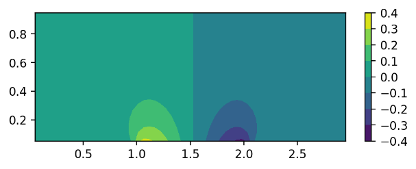
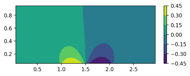
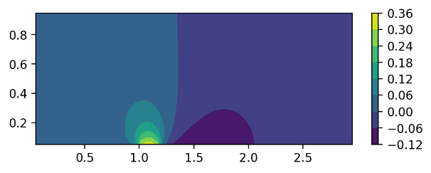
Figure 8. The y-direction velocity distributions of different airfoil shapes. (a) sin function; (b) parabolic function; (c) symmetric triangle function; (d) non-symmetric triangle function.

Figure 8 shows the y-direction velocity distributions of different airfoil shapes, in the same layout as the x-direction velocity distributions. The sin function y-direction velocity distribution, as explained before, is due to the front of the airfoil quickly redirecting air upwards, which then crosses the middle and heads gradually downward as a negative velocity. The parabolic function-shaped airfoil shows similar behaviors, but due to the parabolic function being less steep, the changes in y-direction velocity are less explicit. The general positive increase in velocity in the front and negative decrease in velocity at the back half of the airfoil is shown, but not in the same outstanding magnitude.

The symmetric triangle airfoil also has the same general layout for the velocity distribution but has a direct and abrupt change from a positive increase to a negative decrease in y-direction velocity. The velocity also reaches the largest magnitude values in the symmetric triangle model. This is because the front side of the triangle and the back side of the triangle meet at an abrupt angle, which would therefore abruptly change the airflow. The asymmetric triangle follows the same trend, but because of the shorter front side, the y-direction velocity quickly increases and then evolves into a stable negative velocity after crossing the intersection point of the two sides. The highest y-direction velocity is also the lowest in the asymmetric triangle compared to the other models, due to the shorter front side disallowing greater positive increases in velocity.

4.3. Comparison with Experiments

In this section, we demonstrate the experimental data of the flow visualization over the different airfoil shapes. For the experiments, we have constructed the physical models of the four different airfoils by 3D printing. In the water tunnel, water is flowing at low velocity and the airfoil model has been put into this laminar flow environment. Then, dye is injected into the system to visualize the flow field over the airfoil. As demonstrated in Fig. 9, the flow fields over the four different airfoil shapes simulated in the previous sections have been visualized by the blue color in the experiment. These results show consistent flow fields compared with the CFD simulation results, which further validates the computational results demonstrated previously.

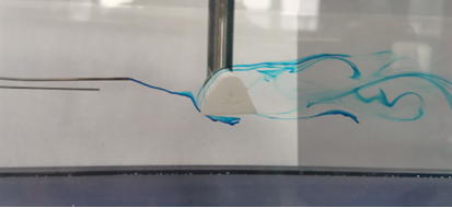
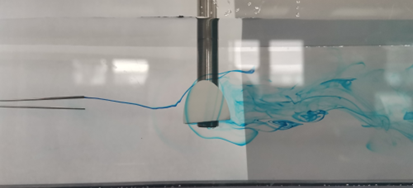
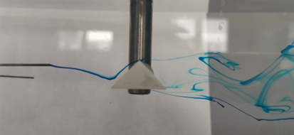
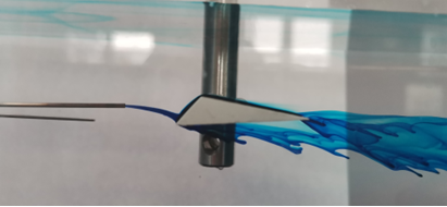
Figure 9. Experimental observations for different airfoil shapes. (a) sin function; (b) parabolic function; (c) symmetric triangle function; (d) non-symmetric triangle function.

5. Conclusion

In this paper, we have performed the CFD simulations of the airfoil by using simplified governing equations. The results show that the flow field (the velocity distributions in both x- and y-directions) over the airfoil has some general trends. Also, the change in the shape of the airfoil could substantially modify the flow field over the airfoil, which is important for the design of aircraft. The simulation results were further compared with the experimental data.

It should be noted that the current work only calculated the 2D flow field over the airfoil. However, for the real aircraft design, the 3D flow fields are needed for the complex fluid dynamics over the airfoil. In the future, the 3D fluid dynamics over airfoil should be simulated using CFD.

In addition, the simulation power of CFD should not be limited to the cases of the airfoil. We could further extend our study to the flow field over other objects by using CFD, for example, racing cars, buildings, and footballs. There are many different situations in which CFD can play an essential role in the design and prediction, which needs to be further explored.

Acknowledgements

I would like to sincerely thank my research supervisor Dr. Wenkai Liang (Princeton University) for his support and guidance during the research process and writing of this paper. I would also like to thank Mr. Zhang for his help with the water tunnel experiments at AUL of SAA, SJTU. Additionally, I would like to thank Dr. Wu for giving some suggestions on revising my paper. Finally, I would like to thank my parents for their continuous support and for helping me stay motivated throughout this research.

References

[1]. Hoffmann, K. A., & Chiang, S. T. (2000). Computational fluid dynamics volume I. Engineering education system.
[2]. Kuzmin, D. (2004). Introduction to computational fluid dynamics. University of Dortmund, Dortmund.
[3]. Hess, J. L. (1990). Panel methods in computational fluid dynamics. Annual Review of Fluid Mechanics, 22(1), 255-274.
[4]. Roache, P. J. (1997). Quantification of uncertainty in computational fluid dynamics. Annual Review of Fluid Mechanics, 29(1), 123-160.
[5]. Versteeg, H. K., & Malalasekera, W. (1995). Computational fluid dynamics. The Finite Volume Method, 1-26.
[6]. Lin, C. L., Tawhai, M. H., Mclennan, G., & Hoffman, E. A. (2009). Computational fluid dynamics. IEEE Engineering in Medicine and Biology Magazine, 28(3), 25-33.
[7]. Ochieng, A., Onyango, M., & Kiriamiti, K. (2009). Experimental measurement and computational fluid dynamics simulation of mixing in a stirred tank: a review. South African Journal of Science, 105(11), 421-426.
[8]. Wexler, D., Segal, R., & Kimbell, J. (2005). Aerodynamic effects of inferior turbinate reduction: computational fluid dynamics simulation. Archives of Otolaryngology–Head & Neck Surgery, 131(12), 1102-1107.
[9]. Kaya, M. N., Kok, A. R., & Kurt, H. (2021). Comparison of aerodynamic performances of various airfoils from different airfoil families using CFD. Wind and Structures, 32(3), 239-248.
[10]. Koziel, S., & Leifsson, L. (2013). Multi-level CFD-based airfoil shape optimization with automated low-fidelity model selection. Procedia Computer Science, 18, 889-898.
[11]. Langtry, R., Gola, J., & Menter, F. (2006, January). Predicting 2D airfoil and 3D wind turbine rotor performance using a transition model for general CFD codes. In 44th AIAA aerospace sciences meeting and exhibit (p. 395).
[12]. Klausmeyer, S. M., & Lin, J. C. (1997). Comparative results from a CFD challenge over a 2D three-element high-lift airfoil (No. NAS 1.15: 112858). National Aeronautics and Space Administration, Langley Research Center.
[13]. McLaren, K., Tullis, S., & Ziada, S. (2012). Computational fluid dynamics simulation of the aerodynamics of a high solidity, small‐scale vertical axis wind turbine. Wind Energy, 15(3), 349-361.
[14]. Piperas, A. T. (2010). Investigation of boundary layer suction on a wind turbine airfoil using CFD. Technical University of Denmark.
[15]. Wolfe, W. P., & Ochs, S. S. (1997). Predicting aerodynamic characteristic of typical wind turbine airfoils using CFD (No. SAND-96-2345). Sandia National Lab.(SNL-NM), Albuquerque, NM (United States).
Cite this article
Bao,H. (2023). Airfoil design with computational fluid dynamics. Theoretical and Natural Science,11,8-18.
Data availability
The datasets used and/or analyzed during the current study will be available from the authors upon reasonable request.
Disclaimer/Publisher's Note
The statements, opinions and data contained in all publications are solely those of the individual author(s) and contributor(s) and not of EWA Publishing and/or the editor(s). EWA Publishing and/or the editor(s) disclaim responsibility for any injury to people or property resulting from any ideas, methods, instructions or products referred to in the content.
About volume
Volume title: Proceedings of the 2023 International Conference on Mathematical Physics and Computational Simulation
© 2024 by the author(s). Licensee EWA Publishing, Oxford, UK. This article is an open access article distributed under the terms and
conditions of the Creative Commons Attribution (CC BY) license. Authors who
publish this series agree to the following terms:
1. Authors retain copyright and grant the series right of first publication with the work simultaneously licensed under a Creative Commons
Attribution License that allows others to share the work with an acknowledgment of the work's authorship and initial publication in this
series.
2. Authors are able to enter into separate, additional contractual arrangements for the non-exclusive distribution of the series's published
version of the work (e.g., post it to an institutional repository or publish it in a book), with an acknowledgment of its initial
publication in this series.
3. Authors are permitted and encouraged to post their work online (e.g., in institutional repositories or on their website) prior to and
during the submission process, as it can lead to productive exchanges, as well as earlier and greater citation of published work (See
Open access policy for details).