1. Introduction

Crime is an important factor that would severely threaten the society. In order to maintain the social security, proper policy should be designed and enforced by the government. In this process, if characteristics of crime, such as reasons, trends, and geographical distribution, could be clearly learned through research based on statistical tool, better policy is more likely to be made and help undermine the crime rate, which could greatly benefit the society.

Several studies have researched the trend of crime rate in the history. According to Tseloini et al, five major types of crime including residential burglary, car theft, theft from cars, personal theft, and assault, declined between 1988 and 2004 in 26 countries based on the data from the International Crime Victim Survey. However, the survey focused on the European and North American countries, which could not show the global trend [1]. Besides the international trend, several studies concentrated on American crime rate. According to Saridakis, from 1960 to 2000, population in the prison and merely social condition had little effect on the violent crime rate; besides, violent crime rate was related to income inequality and racial composition [2]. In the study conducted by Zimring, there was a great decline of American crime rate from 1991 to 2000, taking 1990 as a cut-off point. Specifically, each type of crime decreased by at least 23 percent [3]. Another research tried to study this phenomenon. Gramlich concluded that although the number of property and violent crimes fell a lot, the public believed condition of crimes got worse. In addition, a proportion of crimes were not reported by the police, which might contribute to the great decline [4].

Crime rate is strongly associated with other factors. Greenberg discussed the Cantor-Land approach, which focused on the relationship between crime rate and Unemployment rate. Although unemployed people were motivated to commit crimes for earning, they would also stay at home to protect themselves [5]. Chintrakarn explored the relationship between income inequality and crime rate. Based on the panel analysis, as income inequality rised, people needed more protection, and thus the crime rate would decrease [6]. Light et.al compared the crime rate among illegal immigrants, formal immigrants, and natives. According to the research, undocumented immigrants had lower crime rate compared to the other two categories since they were afraid of being detected as well as hoped for economic success. Therefore, the punishment on illegal immigrants might not affect crime rate. However, the crime rate of the descendants of illegal immigrants was similar to the locals probably due to assimilation theory [7]. Significant global events would also influence the American national crime rate. According to Boman, Covid 19 epidemic caused the overall decline in the crime rate after the government imposed strict restriction to resist the epidemic because lockdown policy prevented group of criminals from committing crime together. However, individual crimes were not affected by Covid 19 [8].

The studies above analyzed the historical trend and the factors contributing to the crime rate. At the same time, forecasting the crime rate is also a very promising field. In this way, this study will analyze different time series models in predicting violent crime rate and find out the most efficient one. Finally, the predicted result could be obtained.

2. Methods

2.1. Data source

In this research, the data on violent crime rate each year is from the Crime Data Explorer on the website of Federal Bureau of Investigation (FBI). The crime rate data in this website is collected from the Summary Reporting System (SRS) and the National Incident-Based Reporting System (NIBRS).

2.2. Data selection

In this research, violent crime rate data from 1991 to 2020 is used to predict the future crime rate. According to the studies of Zimring, 1991 was an important turning point when the crime rate started showing a sharp decreasing trend [9]. In this way, it could be a desirable starting point. At the same time, the crime rate in 2020 is the latest data FBI reports. As a result, this research will use the data before 2020 to predict the violent crime rate from 2021 to 2025 (Fig 1 and Table 1).

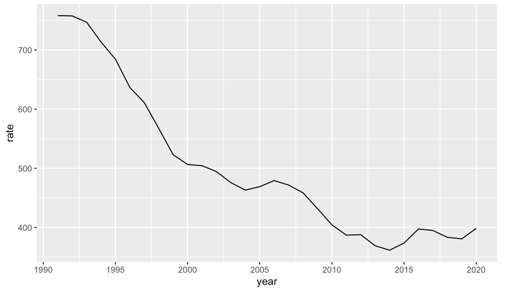
Figure 1. Violent crime rate in each year.

Table 1. Violent crime rate in each year [9].

*Year is the time for the annual violent crime rate data next to it

** Rate is the number of people who commit violent crime per 100,000 people

2.3. Research protocol

This study will test five different approaches to figure out the best one, and they are the average method, naïve method, drift method, linear model, and autoregressive integrated moving average model (Arima model). This research will program in R-Studio to construct the models and check their accuracy, including checking the range and autocorrelation of residuals [10]. Following, the research would use the best model to obtain the future prediction.

2.3.1. The average method. Prediction is equal to the average value of the data set, and the equation is:

\( {\hat{y}_{T+h∣T}}=\bar{y}=({y_{1}}+⋯+{y_{T}})/T \) (1)

2.3.2. The naïve method. Prediction is equal to the latest value in the data set, and the equation is:

\( {\hat{y}_{T+h∣T}}={y_{T+h-m(k+1)}} \) (2)

2.3.3. The drift method. Prediction is based on the average change in historical data, and the equation is:

\( {\hat{y}_{T+h∣T}}={y_{T}}+\frac{h}{T-1}\sum _{t=2}^{T} ({y_{t}}-{y_{t-1}})={y_{T}}+h(\frac{{y_{T}}-{y_{1}}}{T-1}) \) (3)

2.3.4. The linear model. Least-squared regression line would be used for prediction when there is a linear relationship between single predictor x and forecast variable y, and the equation is:

\( {y_{t}}={β_{0}}+{β_{1}}{x_{t}}+{ε_{t}} \) (4)

2.3.5. The Arima model. It is the combination of autoregression and moving average model [10]. In this research, most of the operations would be automatically performed in the R-Studio. Its full model could be written as:

\( y_{t}^{ \prime }=c+{ϕ_{1}}y_{t-1}^{ \prime }+⋯+{ϕ_{p}}y_{t-p}^{ \prime }+{θ_{1}}{ε_{t-1}}+⋯+{θ_{q}}{ε_{t-q}}+{ε_{t}} \) (5)

3. Results and discussion

3.1. Testing of each model

3.1.1. Testing of the average method. According to figure 2, the residuals from the average method varied from -135 to 261, which is very large. Apart from this, the residuals show an evident decreasing trend, which means the model is not effective. According to table 2, by using the Ljung-Box test, the Q*value is extremely high, which means the residuals have a very strong autocorrelation.

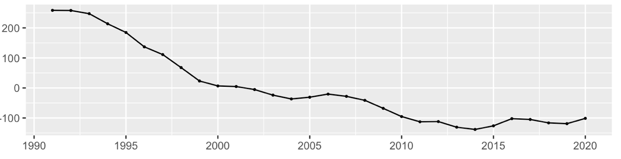
Figure 2. Residuals from the average method.

Table 2. Autocorrelation testing of the average method.

3.1.2. Testing of the naïve method. According to figure 3, the residuals are between -50 and 25, which is not too big. However, the residuals are not randomly distributed below or above the, which means the residuals do not look like white noise. In table 3, when the residuals are checked in the Ljung-Box test, there is a small degree of autocorrelation. When the ACF graph of the residuals is observed in figure 3, although most of the values are lower than the significance level, the value of the first lag is too big, which means there is strong autocorrelation in the first lag.

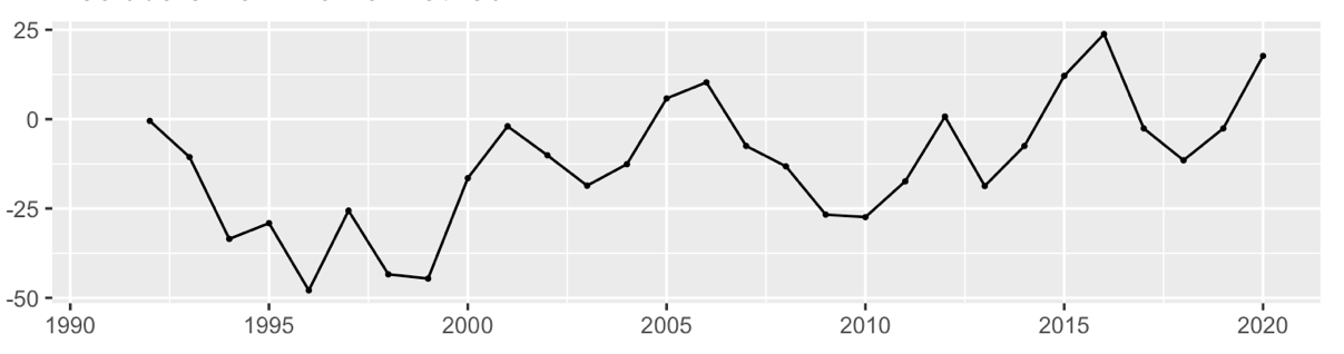
Figure 3. Residuals from the naïve method.

Table 3. Autocorrelation testing of the naïve method.

3.1.3. Testing of the drift method. According to figure 4, the residuals are between -50 and 25, which is not too big. However, a larger proportion of residuals are below 0, which means the residuals do not look like white noise. In addition, based on the Ljung-box test result in table 4, there is a small degree of autocorrelation, and the autocorrelation exists in the first lag.

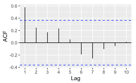
Figure 4. ACF of residuals from the drift method.

Table 4. Autocorrelation testing of the drift method.

3.1.4. Testing of the linear model. Firstly, this research would use R-Studio to find the least-squares regression line between the violent crime rate and the time. The regression line in figure 5 represents the trend of the data. The coefficient of the year corresponding to the violent crime rate is -13.288, which means on average the violent crime rate decreases by 13.288 as one year has passed. Since the P value is lower than 0, the trend is highly significant, which means there is a linear relationship between the year and the violent crime rate. After that, the residuals of the linear model of crime rate will be checked (table 5).

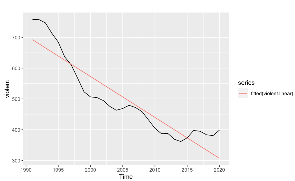
Figure 5. Linear regression result of violent crime rate.

Table 5. Linear regression result of violent crime rate.

In figure 6, the residuals are between -68 and 83, which are relatively large. According to the Breusch-Godfrey test result in table 6, the residuals from the linear models of the violent crime rate are autocorrelated. In addition, the first three lags of the ACF graph are higher than the critical value, showing that within the first lag, autocorrelation is strong.

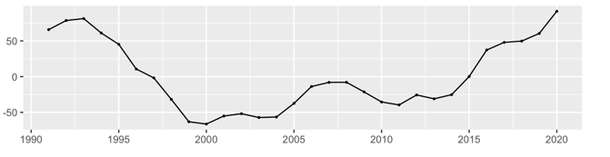
Figure 6. Residuals from the linear method.

Table 6. Autocorrelation testing of the linear model.

3.1.5. Testing of the Arima model. This research would use “auto.arima” in the tool package of R-Studio to find the Arima model with the least residuals, which is Arima (0, 2, 0). When we check the residuals in figure 7, they are nearly randomly distributed above or below 0 between -26 and 28. In this case, it can be shown that the residuals are relatively small and look like white noise. According to the Ljung-Box test in table 7, there is a very small degree of autocorrelation that can be omitted. Apart from this, in figure 8, all the ACF value is lower than the significance level, and the value of the first lag is extremely low (table 7).

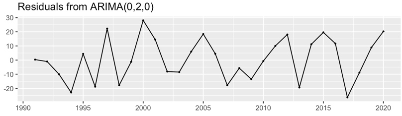
Figure 7. Residuals from the Arima model.

Table 7. Autocorrelation testing of the linear model.

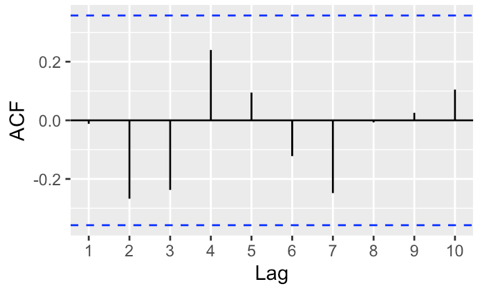
Figure 8. ACF of residuals from the Arima model.

3.2. Selection of models

Based on table 8, the Arima model is the most effective in predicting the American violent crime rate in the future. It has the smallest residuals, and the autocorrelation is negligible, which means it possesses the merits of accurate models. Therefore, this research would use Arima (0, 2, 0) to perform the prediction in the following session.

Table 8. Comparison of different models.

3.3. Prediction results and discussion

Based on table 9, the violent crime rate will increase by 17.7 per 100,000 people, and the prediction is 216.2 in 2021, 233.9 in 2022, 251.6 in 2023, 469.3 in 2024, and 487 in 2025. Since this research is conducted in 2023, the most valuable part should be the prediction in 2024 and 2025.

In figure 9, Arima (0, 2, 0) gives a forecast of increasing violent crime rate from 2021 to 2025, which is different from the long-term trend. In this way, it could be explained that after a sharp decrease of violent crime rate, the rate of the violent crime rate decline decreased gradually but will eventually increase again. In this process, the derivative of the violent crime rate continues to increase so that the model shows a U-shape. Another possibility is that this model may not be fully accurate. Based on the figure, the violent crime rate remains relatively stable from 2011 to 2020, so it may continue to be unchanged rather than start to increase. However, Arima (0, 2, 0) considers the decreasing trend from 1991 to 2010, which will dramatically change the result.

Regardless of the possible errors, this research predicts that the violent crime rate will increase in the following years, which means the condition of violent crime in following years is not as optimistic as the condition in the past thirty years. Therefore, the government should pay more attention to the violent crime. For example, the government should increase its expenditure on social security or call on the community to prevent violence from happening, which could effectively undermine criminals.

Table 9. Predicted value of violent crime rate.

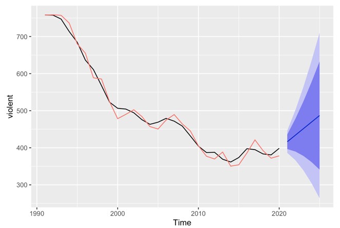
Figure 9. The prediction of Arima(1,2,0).

4. Conclusion

Previous studies explored the historical trend of crime rate: the number of all types of crimes declined dramatically after 1990. In addition, some studies showed that the crime rate is related to certain factors such as unemployment rate, income inequality, immigrants, and influential events. However, this research study focuses on one type of crime, violent crime, predicting its future change based on time series analysis. Within the five candidate models, Arima (0, 2, 0) shows the highest accuracy. It has negligible autocorrelation and the smallest residuals, so it could be used in the prediction in this research.

The prediction of the violent crime rate shows an increasing trend in the following models, which contradicts the long-term trend after 1990. In this case, this research recommends the government to take violent crime seriously, taking action to prevent the happening of violent crime.

References

[1]. Bai J J 2022 Method and Application of Calculating Comprehensive Crime Rate. Chinese Journal of Criminal Law, 55.
[2]. Saridakis G 2004 Violent crime in the United States of America: A Time-series analysis between1960–2000. European Journal of Law and Economics, 18, 203-211.
[3]. Guo D M, et al. 2021 Housing prices, wealth inequality, and urban crime rate: an empirical analysis based on panel data of prefecture level cities in Chin. Journal of Central University of Finance and Economics, 113-128.
[4]. Greenberg D F 2001 Time series analysis of crime rates. Journal of quantitative criminology, 17, 291-327.
[5]. Chintrakarn P and Herzer D 2012 More inequality, more crime? A panel cointegration analysis for the United States. Economics Letters, 116(3), 389-391.
[6]. Light M T, He J and Robey J P 2020 Comparing crime rates between undocumented immigrants, legal immigrants, and native-born US citizens in Texas. Proceedings of the National Academy of Sciences, 117(51), 32340-32347.
[7]. Boman J H and Gallupe O 2020 Has COVID-19 changed crime? Crime rates in the United States during the pandemic. American journal of criminal justice, 45, 537-545.
[8]. Zhang P and Yang F 2022 The Impact of Urban Settlement Threshold on the Crime Rate of Floating Population. Population and Society, 38(3), 13.
[9]. Hong Y and Yuan X X 2023 Regional Income Gap, Population Mobility, and Criminal Crime Rate. Southern Population, 38(1), 46-58.
[10]. Xie X Y and Zhou Y 2022 Preliminary Study on the Comparison of International Re crime Rate Data. Journal of Henan Judicial Police Officer Vocational College, 20(1), 7.
Cite this article
Yang,M.H. (2023). The research of prediction of future violent crime rate. Theoretical and Natural Science,26,192-200.
Data availability
The datasets used and/or analyzed during the current study will be available from the authors upon reasonable request.
Disclaimer/Publisher's Note
The statements, opinions and data contained in all publications are solely those of the individual author(s) and contributor(s) and not of EWA Publishing and/or the editor(s). EWA Publishing and/or the editor(s) disclaim responsibility for any injury to people or property resulting from any ideas, methods, instructions or products referred to in the content.
About volume
Volume title: Proceedings of the 3rd International Conference on Computing Innovation and Applied Physics
© 2024 by the author(s). Licensee EWA Publishing, Oxford, UK. This article is an open access article distributed under the terms and
conditions of the Creative Commons Attribution (CC BY) license. Authors who
publish this series agree to the following terms:
1. Authors retain copyright and grant the series right of first publication with the work simultaneously licensed under a Creative Commons
Attribution License that allows others to share the work with an acknowledgment of the work's authorship and initial publication in this
series.
2. Authors are able to enter into separate, additional contractual arrangements for the non-exclusive distribution of the series's published
version of the work (e.g., post it to an institutional repository or publish it in a book), with an acknowledgment of its initial
publication in this series.
3. Authors are permitted and encouraged to post their work online (e.g., in institutional repositories or on their website) prior to and
during the submission process, as it can lead to productive exchanges, as well as earlier and greater citation of published work (See
Open access policy for details).