1. Introduction

Research and Markets 2023 Global Market Report for Real Estate Agents and Brokers predicts a compound annual growth rate of 7.3% in the global real estate agency market, which is projected to increase from $1.32 trillion in 2022 to $1.4 trillion in the same year. This growth highlights the importance of understanding the factors that influence housing prices, as it provides essential insight into the worth of homes and the sentiment of buyers and sellers. Predicting housing prices accurately and identifying the key factors that drive these prices is crucial for various stakeholders in the real estate market, including homeowners, real estate agents, and property developers. This study focuses on predicting home prices in Ames, Iowa, using two regression techniques: forward selection regression and principal component regression. The objective is to develop reliable predictive models that can accurately estimate a house’s price based on essential information. Additionally, these models should offer insights into the factors that significantly impact housing prices, revealing the attributes of a property that are most closely tied to its value. To achieve this objective, the research begins with exploratory data analysis and several data preprocessing steps. Features are classified, overlapping features are merged, missing values are appropriately handled, and predictors with zero or near-zero variance are removed. The data is then scaled to address any issues related to data fragmentation. By employing these regression techniques and analyzing the data, this study aims to provide valuable guidance for stakeholders in the real estate market. Homeowners, real estate agents, and property developers can benefit from the identified factors that contribute significantly to the value of real estate in Ames, Iowa. This research can help stakeholders make informed decisions to enhance their investments and improve the value of their properties.

2. Literature Review

A plethora of research has been done on forecasting housing prices, employing a range of methods such as linear regression, decision trees, and machine learning algorithms. Rosen (1974) introduced the concept of hedonic pricing models, which use observed characteristics of a good to estimate its implicit price. Widely employed to forecast housing costs, Malpezzi (2003) [1] has employed this technique.

Moreover, Machine learning techniques show promise in housing price prediction. Celik et al. (2012) used artificial neural networks (ANN) for predicting housing prices in Istanbul and found that ANNs outperformed multiple linear regression [2]. Park and Bae (2015) employed random forests in Gyeonggi Province, South Korea, and showed that their model outperformed linear regression, decision tree, and k-nearest neighbors’ models [3].

Selecting features is a fundamental part of constructing predictive models, as it helps to simplify the model, avoid overfitting, and enhance its interpretability. Guyon and Elisseeff (2003) gave an overview of filter techniques and showed their use in a variety of areas. Filter techniques evaluate the importance of each feature separately, based on statistical metrics such as correlation or mutual data [4]. For example, Tsai and Chen (2014) used filter methods, specifically correlation-based feature selection, to identify relevant features for predicting housing prices in Taiwan. The dataset [5] revealed that the location, land area, and age of the building were the most essential elements in determining housing prices.

Kohavi and John (1997) pioneered a wrapper technique for feature selection, which assesses subsets of features by constructing models and gauging their efficacy [6]. Mao et al. (2011) then employed a wrapper approach, particularly forward stepwise selection, to identify the most pertinent features for forecasting housing prices in Beijing. Their results showed that variables like the floor area ratio, distance to the central business district, and green coverage ratio were significant predictors of housing prices [7].

For regression techniques, linear regression has been a popular choice for housing price prediction due to its simplicity and interpretability. In 1986, Frew and Jud investigated the correlation between housing costs and a variety of socioeconomic elements in the United States [8]. Can (1992) then investigated the influence of housing features, ecological benefits, and local characteristics on house prices in the US, discovering that these elements significantly impacted housing prices [9]. In addition, Li et al. (2016) applied principal component regression (PCR) to predict house prices. By blending Principal Component Analysis (PCA) and Linear Regression, PCR is a method employed to tackle multicollinearity issues in the data set. Li and colleagues used this method to predict housing prices in China and demonstrated that PCR provided more accurate predictions than traditional multiple linear regression [10].

While previous studies have applied various regression techniques for housing price prediction, a direct comparison of forward stepwise selection and PCR has not been extensively explored. Additionally, these techniques have not thoroughly investigated the Ames Housing dataset. This study aims to fill these gaps by applying forward stepwise selection and PCR to the Ames Housing dataset and comparing the performance of the two models.

3. Data and Methodology

The purpose of this research is to forecast housing costs in Ames through two techniques: forward selection regression and principal component regression (PCR).

3.1. Data

3.1.1. Description of Data. The Ames Housing Dataset, compiled by Dean De Cock in 2011, presents data about 2930 residential real estate transactions that took place in Ames, Iowa, U.S., between 2006 and 2010. This set of information is widely seen as an enhanced and updated variant of the well-known Boston Housing Dataset and hence, was selected for this investigation. The dataset for training encompasses 1460 instances and 79 predictor variables, where the “Sale Price” serves as the dependent variable. The dataset was originally sourced from Kaggle.

3.1.2. Data processing. The research was conducted with Exploratory Data Analysis (EDA), proceeding through various data preprocessing steps. We first categorize the features. There are four main categories: environment, configuration, properties, and scoring. The results are shown in Table 1.

Table 1. Classification of data.

The dataset exhibits numerous features that possess shared characteristics. For instance, the general state of a house is expressed through both “Overall Quality” and “Overall Condition”. By integrating these shared features, it’s possible to decrease noise within the dataset. Hence, this investigation has merged “Overall Quality” and “Overall Condition” to establish a unified feature. This method was also implemented on the pairs of features, “Garage Quality” & “Garage Condition,” “Exterior Quality” & “Exterior Condition,” and “Basement Quality” & “Basement Condition.”

Divide the absent values into two distinct groups. One category is true missing data, and the other category is “NA” which is meaningful. For the 15 predictors where NA has a specific meaning (Alley, BsmtQual, BsmtCond, BsmtExposure, BsmtFinType1, BsmtFinType2, FireplaceQu, GarageType, GarageFinish, GarageQual, GarageCond, PoolQC, Fence, MiscFeature, GarageYrBlt), there is no need to imputation NA as a missing value. Assign a value of 0 to a predictor that has a specific meaning for NA. For the truly missing predictor, remove them.

The data is digitized using the ‘as. integer’ function. The predictors of zero and near-zero variance are then removed. Some redundant features are shown in Figure 1.

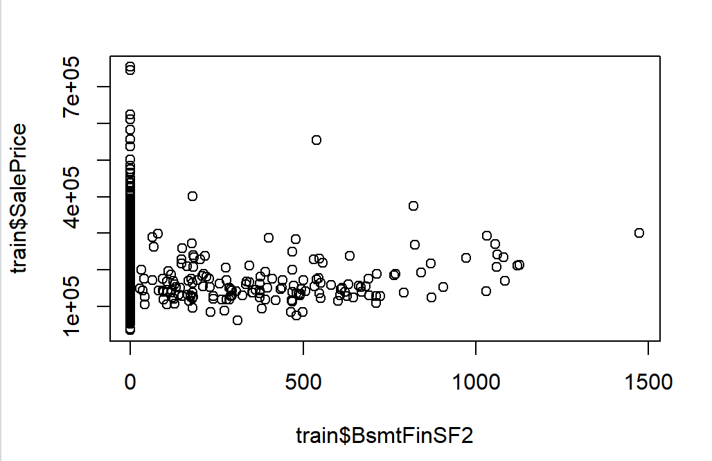
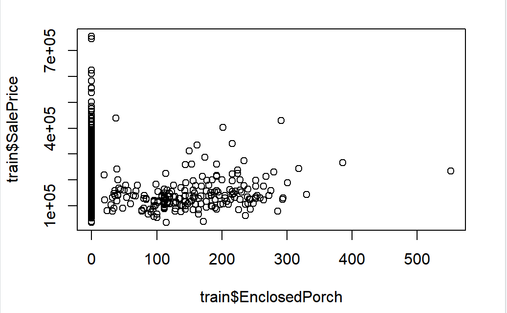
Figure 1. Redundant features: Observations are limited to the same value or category.

After that, the data needs to be scaled because the data is scattered. Some data that has not been standardized is shown in Figure 2.

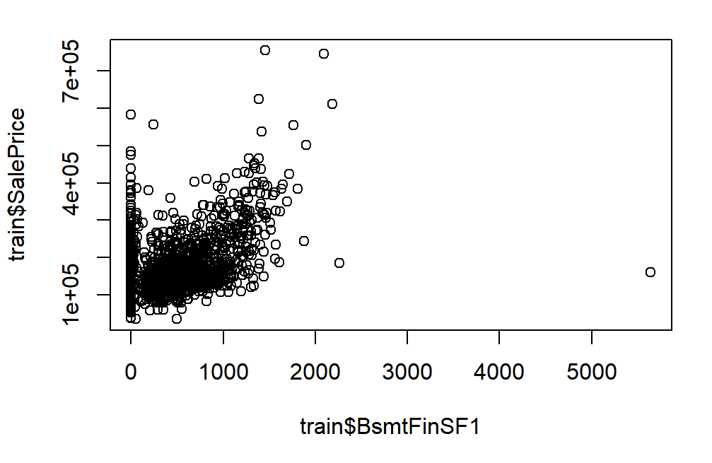
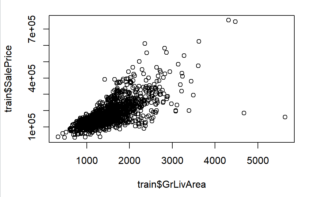
Figure 2. Some data that has not been standardized.

This study displays the data as a typical normal distribution. The process is undertaken by ‘preProcess ()’ in Caret.

After that, multicollinearity was removed from the data, and variables significantly correlated with the target variable “SalePrice” at a given significance level of 0.05 were screened out.

3.2. Methodology

3.2.1. Forward selection regression. Regression forward selection is a technique of feature selection that begins with an empty model and adds features to find the most pertinent predictors for the target variable. At each step, the predictor which yields the most significant improvement in the model’s goodness-of-fit is chosen. This process continues until no significant improvement is seen by adding more predictors or a predefined stopping criterion is met.

Forward selection regression can be employed to pinpoint the most critical features that shape housing prices, such as location, size, and age of the property. By only including pertinent predictors in the model, it can simplify the model, avoid overfitting, and enhance interpretability.

RMSE, a measure of model accuracy, is used in this study. A higher RMSE value implies a greater model accuracy. Let us assume the observed values are \( {y_{1}}{, y_{2}},……, {y_{k}} \) , and the predicted values are \( \hat{{y_{1}}}, \hat{{y_{2}}}, ……, \hat{{y_{k}}} \) . This is determined by computing the square root of the mean square error (MSE):

\( RMSE=\sqrt[]{MSE}= \) \( \sqrt[]{\frac{\sum _{i}{( yi-\hat{{y_{i}}})^{2}}}{n}} \) (1)

where:

n is the number of observations in the dataset (nrow(train)).

Adjusted R2 is used to evaluate the statistically significant enhancement level. This is a way to gauge the accuracy of the regression equation. Unlike the regular R-squared, which increases with the addition of more predictors to the model, adjusted R-squared takes into consideration the number of predictors and adjusts the value accordingly. This helps to find a model that balances complexity and fit and prevents overfitting. The formula for adjusted R-squared is as follows:

(2)

where:

\( {R^{2}}= \) \( \frac{\sum _{i}{( \hat{{y_{i}}}-\bar{y})^{2}}}{\sum _{i}{({y_{i}}-\bar{y})^{2}}} \) (3)

n is the number of observations (samples). p is the number of predictors (features).

3.2.2. Principal Component Regression (PCR). By combining Principal Component Analysis (PCA) and linear regression, Principal Component Regression (PCR) is a method to tackle multicollinearity issues in the dataset. PCA is a dimensionality reduction technique that transforms the original predictors into a new set of uncorrelated variables, known as principal components. These components can capture the greatest amount of variance in the original data while preserving orthogonality.

In PCR, the first step is to perform PCA on the predictor variables, and then a linear regression model is fit using the principal components as the new predictors. By using PCR, the model can handle multicollinearity issues caused by correlated predictors and achieve more accurate predictions than traditional multiple linear regression.

4. Results

4.1. Model selection

4.1.1. Forward selection regression. The forward stepwise selection was achieved using library ‘leaps’, selecting the best model based on the maximum adjusted R-squared value. The RMSE for the best model is then calculated to assess its accuracy. The relationship between the number of variables and the adjusted R-squared value is shown in Figure 3.

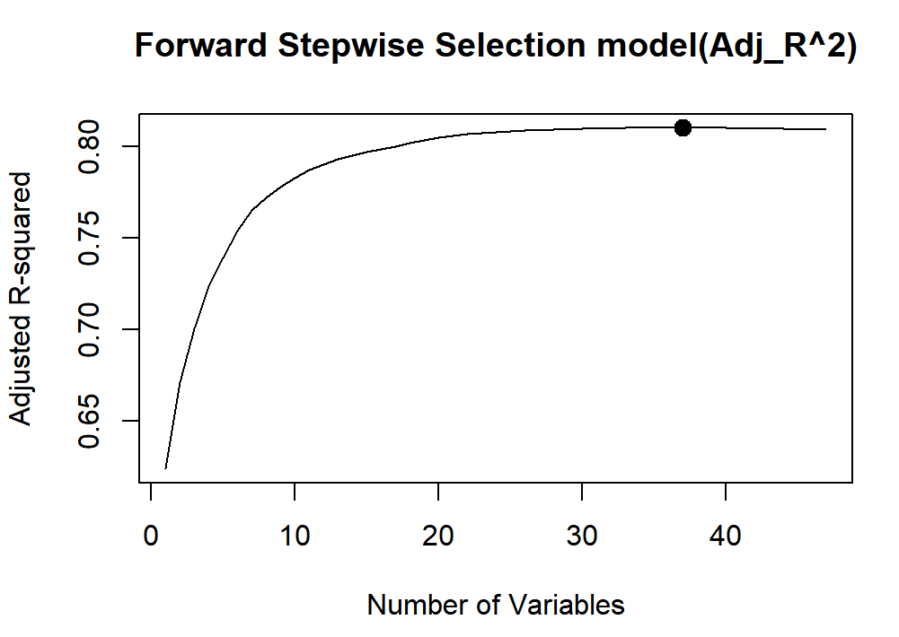
Figure 3. The relationship between the number of variables and the adjusted R-squared value.

When number of variables is 37, R squared is the largest. 37 variables are shown in Figure 4:

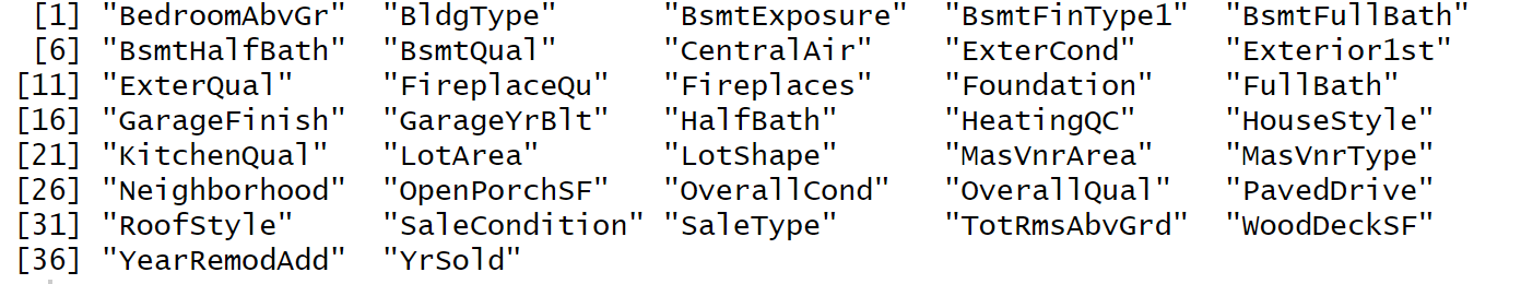
Figure 4. 37 variable names.

Figure 5 illustrates the significance of the pertinent variables, with only the top 20 chosen for presentation.

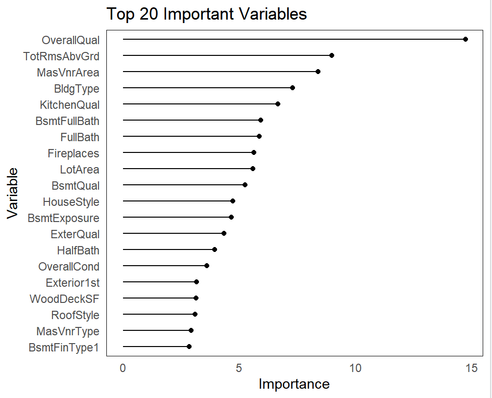
Figure 5. The significance of the pertinent variables.

Now the RMSE is 0.116.

4.1.2. Principal Component Regression (PCR). Cross-validation was employed in this research to find the minimal RMSE by determining the number of primary components. Finally, it is decided that the RMSE is the smallest when the Number of components is 47, and the RMSE is 0.231. Figure 6 illustrates the significance of principal component-related variables, with only the top 20 chosen for display.

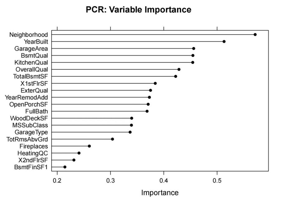
Figure 6. The significance of principal component-related variables.

4.2. Evaluation model

Forward selection regression, due to its lower RMSE, is chosen to construct a multiple linear regression model. Figure 7 displays the comparison between the real data of the training set and the predicted data.

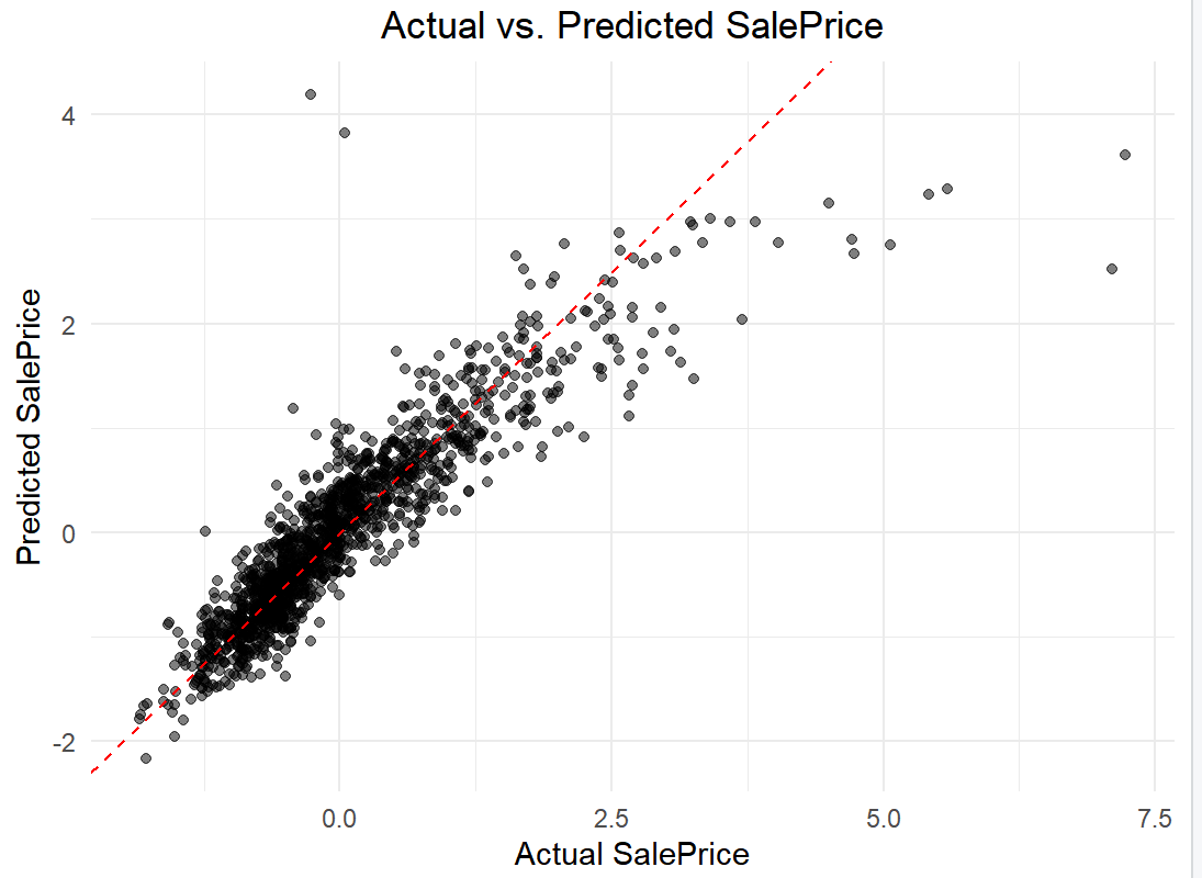
Figure 7. The comparison between the real data of the training set and the predicted data.

4.3. Prediction Results of Linear Regression

Use forward selection regression to make predictions about the test set. SalePrice is automatically predicted by using the ‘predict’ function. Some of the results after regularization are shown in Figure 8:

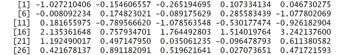
Figure 8. The results after regularization.

5. Discussion

The main concentration of the discourse is on the efficacy of forward selection regression and Principal Component Regression (PCR) in forecasting house prices, as well as their disparities in finding variable significance.

Firstly, it is noteworthy that forward selection regression and PCR show different performances in predicting house prices. The forward selection regression’s RMSE value of 0.116 implies a more exact prediction of house prices. However, the RMSE value of PCR is higher (0.231), which might be due to its sacrifice of some predictive accuracy when dealing with multicollinearity issues.

Secondly, the differences in figuring out variable importance between the two methods are also significant points of discussion. The adjusted R-squared value figures out the significance of 37 variables chosen in forward selection regression, whereas PCR selects 47 principal components, the RMSE value being the deciding factor. This disparity between the two approaches could be the cause of their divergent outcomes in forecasting house prices.

In addition, this study has drawn several insights.

(1) Both models emphasized the importance of the predictive factors “OverallQual” and “KitchenQual”, ranking them among the top six. This shows that the overall material and finish of the house, particularly the kitchen, greatly impact the value of the house. This might be somewhat surprising, suggesting that real estate market participants should pay more attention to the kitchen area.

(2) Apart from “OverallQual” and “KitchenQual”, other predictive factors also played significant roles. For instance, the quality of the basement and the condition of the bathrooms ranked relatively high on the variable importance measurement chart.

According to the above analysis, this study suggests that choosing the proper prediction method and method for determining variable importance is crucial for the accuracy of house price prediction. Exploration of other prediction techniques and variable selection approaches could be further investigated to improve the precision of house price forecasting.

6. Conclusions

In this study, the researchers conducted exploratory data analysis and various data preprocessing steps to process the dataset. These steps included categorizing features, consolidating overlapping ones, handling missing values, and scaling the data. By categorizing and consolidating features, the researchers were able to reduce noise within the dataset and improve its quality. Additionally, handling missing values and scaling the data helped to ensure the accuracy and consistency of the dataset.

The study focused on predicting house prices using the forward selection regression method. The results showed that this method had higher prediction accuracy and a lower root mean square error (RMSE) value compared to other regression techniques. This indicates the superiority of the forward selection regression method in predicting house prices.

Furthermore, the study identified several important factors that significantly impact house prices. Notably, “OverallQual” and “KitchenQual” have been identified as significant factors. This finding emphasizes the impact of a house’s overall material and finish, particularly the kitchen, on its value. Other factors, like the quality of the basement and the condition of the bathrooms, were also found to be significant. These findings provide valuable insights into the factors that influence housing prices and can be used by stakeholders in the real estate market to make informed decisions and enhance their investments.

Overall, this study contributes to the understanding of housing price prediction and provides practical guidance for homeowners, real estate agents, and property developers. By focusing on the identified factors that contribute significantly to the value of real estate, stakeholders can make informed decisions to enhance their investments and improve the value of their properties.

References

[1]. S. Malpezzi, “Hedonic pricing models: a selective and applied review”, Housing economics and public policy, vol. 1, pp. 67-89, 2003.
[2]. Ö. Çelik, A. Teke, and H. B. Yıldırım, “Real estate appraisal using artificial neural networks”, Journal of Civil Engineering and Management, vol. 18, no. 6, pp. 845-856, 2012.
[3]. B. Park and J. K. Bae, “Using machine learning algorithms for housing price prediction: The case of Fairfax County, Virginia housing data”, Expert Systems with Applications, vol. 42, no. 6, pp. 2928-2934, 2015.
[4]. I. Guyon and A. Elisseeff, “An introduction to variable and feature selection”, Journal of Machine Learning Research, vol. 3, no. Mar, pp. 1157-1182, 2003.
[5]. R. Kohavi and G. H. John, “Wrappers for feature subset selection”, Artificial Intelligence, vol. 97, no. 1-2, pp. 273-324, 1997.
[6]. C. F. Tsai and M. Y. Chen, “A data mining-based approach for the prediction of real estate business cycle turning points”, Applied Economics, vol. 46, no. 12, pp. 1319-1328, 2014.
[7]. Q. Mao, J. Huang, H. Cao, and C. Wang, “Prediction of Beijing housing prices based on wrapper feature selection”, in 2011 Int. Conf. Manage. Service Sci., pp. 1-4, 2011.
[8]. J. R. Frew and G. D. Jud, “The specification of hedonic housing price models”, AREUEA Journal, vol. 14, no. 3, pp. 386-401, 1986.
[9]. A. Can, “Specification and estimation of hedonic housing price models”, Regional Science and Urban Economics, vol. 22, no. 3, pp. 453-474, 1992.
[10]. H. Li, Y. D. Wei, C. Wu, and G. Tian, “Analyzing housing prices in Shanghai with open data: Amenity, accessibility, and urban structure”, Cities, vol. 56, pp. 48-61, 2016.
Cite this article
Wang,Z. (2024). Research on predicting Ames housing price based on forward selection regression and principal component regression. Applied and Computational Engineering,45,92-101.
Data availability
The datasets used and/or analyzed during the current study will be available from the authors upon reasonable request.
Disclaimer/Publisher's Note
The statements, opinions and data contained in all publications are solely those of the individual author(s) and contributor(s) and not of EWA Publishing and/or the editor(s). EWA Publishing and/or the editor(s) disclaim responsibility for any injury to people or property resulting from any ideas, methods, instructions or products referred to in the content.
About volume
Volume title: Proceedings of the 4th International Conference on Signal Processing and Machine Learning
© 2024 by the author(s). Licensee EWA Publishing, Oxford, UK. This article is an open access article distributed under the terms and
conditions of the Creative Commons Attribution (CC BY) license. Authors who
publish this series agree to the following terms:
1. Authors retain copyright and grant the series right of first publication with the work simultaneously licensed under a Creative Commons
Attribution License that allows others to share the work with an acknowledgment of the work's authorship and initial publication in this
series.
2. Authors are able to enter into separate, additional contractual arrangements for the non-exclusive distribution of the series's published
version of the work (e.g., post it to an institutional repository or publish it in a book), with an acknowledgment of its initial
publication in this series.
3. Authors are permitted and encouraged to post their work online (e.g., in institutional repositories or on their website) prior to and
during the submission process, as it can lead to productive exchanges, as well as earlier and greater citation of published work (See
Open access policy for details).