1. Introduction

House price prediction is a significant field within the domain of real estate and finance. It involves utilizing statistical modeling and machine learning techniques to forecast the prices of residential properties. The objective of house price prediction is to provide accurate estimates of property values, which are valuable for various stakeholders including homebuyers, sellers, investors, and financial institutions.

The background of house price prediction can be traced back to the emergence of real estate markets and the need to assess property values. Traditionally, real estate appraisers and agents relied on their expertise and market knowledge to estimate house prices. However, with the advent of technology and the availability of large datasets, predictive modeling techniques have gained prominence.

The availability of extensive housing data, such as property features, location, historical prices, economic indicators, and demographic factors, has enabled the development of sophisticated predictive models. These models utilize various algorithms, including linear regression, decision trees, random forests, support vector machines, and more recently, deep learning methods like neural networks.

This research is going to figure out what key factors can influence the house price, make comparisons between different models and give some recommendations for people.

2. Literature Review

The essays referred to in this research are mostly found at https://www.cnki.net, which is the official website of essays published in China. And the other essays are found in the reference list of these essays.

In real production applications, there will be certain errors or missing data, or it does not meet the needs of the model. Poor quality data often leads to poor efficiency of data modeling, and even directly leads to severe problems such as significant errors in the model. In order to ensure the validity of the data and make it meet the application requirements, appropriate data preprocessing should be carried out at the beginning of the model building.[1]

When modeling, emphasis is placed on finding correlations between data and verifying them. At the same time, the use of data to avoid the occurrence of data islands, the need for data correlation operations, and the purpose of correlation analysis is to test the covariance trend of two random variables. For regression analysis, the dependent variable must be a random variable, while the independent variable can be either a common variable or a random variable, which will not have a fundamental impact on the experimental results.

Support vector machine (SVM) is a new general learning method developed in 1995 based on the theory of statistical learning. It solves the problems of structure selection and local minimum (overfitting, underfitting) of the second-generation neural network. SVM, which is based on statistical learning theory, has been applied to various fields of machine learning and is called the most general universal classifier.[2]

The random forest model is often used in classification and regression problems. In the classification problem, the random forest combines multiple decision trees and then votes to obtain the final classification result.[3]

Extreme Gradient Boosting (XGBoost) is proposed by Dr. Chen Tianqi [4], an integrated machine learning algorithm based on the decision tree (GBDT). The fundamental idea of XGBoost is to train multiple weak decision trees in series to form a strong decision tree. Each decision tree may not have a good classification effect, but multiple decision trees will get more accurate results. This model is suitable for classification and regression problems and has obvious advantages over traditional models, such as fast training, low cost, and low generalization error.

The idea of the XGBoost algorithm is to continuously add trees, each feature split will add a new tree, and each new tree will use a new function to fit the last predicted residual. When the training is completed, K trees will be obtained. Predicting the score of a sample is based on the characteristics of this sample, each tree will fall into its corresponding leaf node, each leaf node corresponds to a score, and finally add up the scores corresponding to each tree to the predicted value of the sample.[5]

3. Methodology

3.1. Data collection

The dataset used in the prediction is downloaded from Kaggle. The source of the dataset: https://www.kaggle.com/code/emrearslan123/house-price-prediction/input.

3.2. Data introduction

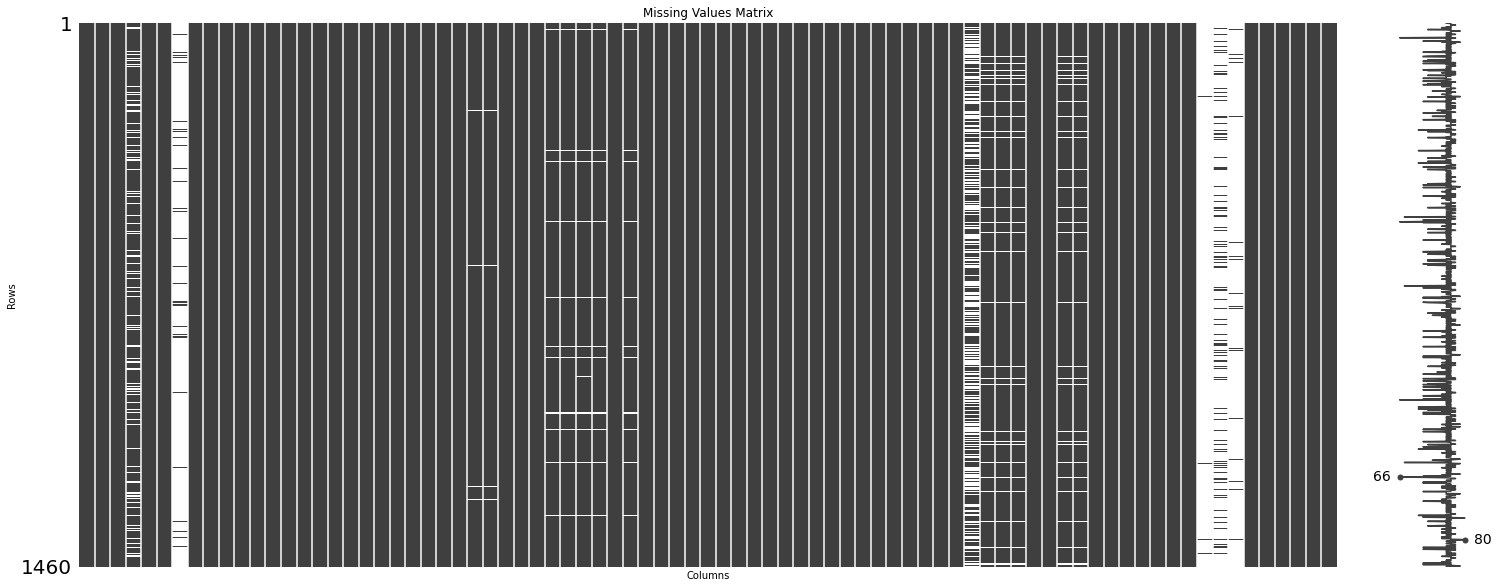
The dataset has 81 columns and 1460 rows, which means there are 81 features of the houses and 1460 houses are recorded. There exist some features with huge amounts of missing values. The count of missing values is shown in Figure 1. If necessary, these features should be dropped. And some features with only a few missing values will be filled with mean or median according to the situation.

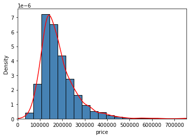
The details of the Sale Price are shown in Table 2. The minimum price of the house is 34900 dollars and the maximum is 755000 dollars in the dataset.

Table 1. Details of the Sale price.

The distribution of the price can be seen in Figure 2. Most house prices are around 150000 dollars, and there is only one peak.

3.3. Data processing

A heatmap is a graphical representation of data where values are encoded as colors in a two-dimensional matrix. It is a way to visualize and explore relationships between two variables, often displayed as a grid of cells, where each cell is filled with a color representing the value of the corresponding data point. A heat map of the dataset is shown in Figure 3.

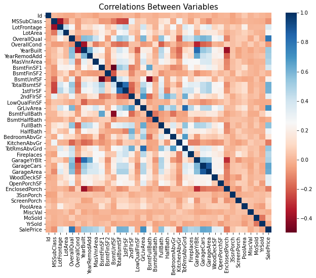
Many features have a low correlation with the Sale price. So, only important features and features with high correlation are picked out. The picked-out features are shown in Table 2.

Table 2. Description of important features.

In this step, it is figured out what are the key factors that are probably influencing the house price.

3.4. Model fitting

In this research, four different models will be used to fit the data and be compared.

Linear regression is a simple and widely used regression model that aims to establish a linear relationship between the independent variables and the dependent variable. It assumes a linear equation where the dependent variable is a linear combination of the independent variables.

Random y with x1, x2, ... The linear regression model for xk is as follows:

\( y={β_{0}}+{β_{1}}{x_{1}}+{β_{2}}{x_{2}}+,...,+{β_{k}}{x_{k}}+ε \)

Where β0, β1, β2, ..., βk is the k+1 location parameters, β0 is called the regression constant β1, β2, ..., βk is called the regression coefficient. y is called the explained variable, x1, x2, ..., xk are k exactly controllable general variables called explanatory variables.[2]

Support Vector Machines is a versatile machine learning algorithm that can be used for both classification and regression tasks. In the context of regression, SVM aims to find a hyperplane that maximizes the margin between the predicted values and the actual values. It uses support vectors, which are the data points closest to the hyperplane, to define the regression line.

The main steps and mathematical theory of the algorithm are as follows.

a. Computation of maximum margin hyperplane; b. Lagrange multiplier; c. K TT condition and dual transformation; d. High-dimensional mapping; e. Kernel functions and soft margins.

By implementing the above steps and mathematical principles, the linear classifier can be applied to nonlinear data sets.[2]

The corresponding regression estimation function is as follows:

\( f(x)=\sum _{{x_{i}}ϵsv}({α_{i}}-α_{i}^{*})K({x_{i}},{x_{j}})+b \)

Where: C>0 is the penalty coefficient, and a larger C means a larger penalty for data points outside the pipeline ε. αi, αi* are the Lagrange multipliers. . 0≤αi≤C,0≤αi*≤ C, the xi corresponding to non-simultaneously zero αi, αi* is the support vector (SV). 0<αi<C, αi*=0; 0<αi*<C, αi =0, the xi corresponding to 0 is the standard support vector (NSVM).

K(xi,xj) = ϕ(xi)ϕ(xj) is called the kernel function.[6]

\( b=\frac{1}{{N_{NSV}}}\lbrace \sum _{0 \lt {α_{i}} \lt c}[{y_{i}}-\sum _{{x_{j}}ϵsv}({α_{j}}-α_{j}^{*})K({x_{j}},{x_{i}})-ε]+\sum _{0 \lt α_{i}^{*} \lt c}[{y_{i}}-\sum _{{x_{j}}ϵsv}({α_{j}}-α_{j}^{*})K({x_{j}},{x_{i}})+ε]\rbrace \)

Random Forest is an ensemble learning method that combines multiple decision trees to make predictions. In the case of regression, a Random Forest Regressor constructs a collection of decision trees and averages their predictions to provide the final output.

The basis and condition for feature selection in decision trees are that entropy decreases the fastest and improves the purity of the data set. The CART tree calculates the effect of each variable on the heterogeneity of the observations at each node of the decision tree using the Gini index. Lower values of the Gini index indicate higher purity. [7] If the selected attribute is A, then the Gini index of the split data set D is calculated as follows:

\( {Gini_{A}}(D)=\sum _{j=1}^{k}\frac{|{D_{j}}|}{|D|}Gini({D_{j}}) \)

XGBoost (Extreme Gradient Boosting) is a popular machine learning algorithm that is widely used for both regression and classification tasks. XGBoost regression specifically refers to the application of XGBoost for regression problems. Regression is a supervised learning task where the goal is to predict a continuous target variable based on input features. XGBoost regression, like other regression algorithms, aims to find a mathematical relationship between the input variables (features) and the target variable, allowing us to make predictions for new data points.

Similar to CART trees, the score values of multiple weak regression trees are summed as the predicted value. Final objective function:

\( obj=\sum _{j=1}^{T}((\sum _{i∈{I_{j}}}{g_{i}}){w_{j}}+\frac{1}{2}(\sum _{i∈{I_{j}}}{h_{i}}+λ)w_{j}^{2})+γT \)

Where j represents the jth regression tree, w regression tree weight, Ij essentially represents a set, each value in the set represents the serial number of a training sample, and the whole set is the training sample divided by the tth CART tree into the jth leaf node.[1]

3.5. Model comparison

In the evaluation and comparison stage, four attributes, which are Mean Absolute Error, Mean Squared Error, Root Mean Squared Error, and R squared, will be used to evaluate the models. The formulas are listed in Table 3.

Table 3. Formula.

MAE (Mean Absolute Error): MAE measures the average absolute difference between the predicted values and the true values. It provides a measure of how close the predictions are to the actual values. MAE is useful when you want to have a metric that is easy to interpret in the original unit of the target variable.

MSE (Mean Squared Error): MSE measures the average squared difference between the predicted values and the true values. It gives more weight to large errors due to the squaring operation. MSE is commonly used in regression tasks and is useful for penalizing larger errors than MAE.

RMSE (Root Mean Squared Error): RMSE is the square root of MSE. It provides a measure of the standard deviation of the residuals or prediction errors. RMSE is also commonly used in regression tasks and has the advantage of being in the same unit as the target variable, making it more interpretable.

R² (R-Squared): R² is a statistical measure that represents the proportion of the variance in the dependent variable (target variable) that can be explained by the independent variables (features) in the regression model. It indicates the goodness of fit of the model. R² ranges between 0 and 1, where 0 indicates that the model does not explain any of the variability in the target variable, and 1 indicates a perfect fit where the model explains all the variability.

4. Result

4.1. Linear Regression

The predicted result compared with the actual is shown in Figure 4.

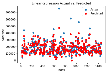
The linear regression model achieves an MAE of 23,567.89, indicating that, on average, the predictions deviate from the true values by approximately 23,567.89 units. The MSE is 1,414,931,404.63, and the RMSE is 37,615.57, suggesting that the model has a moderate level of error. The R² score of 0.8155 indicates that approximately 81.55% of the variance in the target variable is explained by the features included in the model. Overall, the linear regression model shows decent performance, but there is room for improvement.

4.2. Support Vector Regression (SVR)

The predicted result compared with the actual is shown in Figure 5.

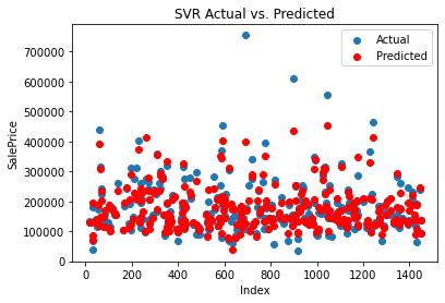
Figure 5. Result of SVR.

The SVM regression model performs slightly better than linear regression, with an MAE of 17,843.16. This suggests that the average deviation of the predictions from the true values is approximately 17,843.16 units. The MSE is 1,132,136,370.34, and the RMSE is 33,647.23, indicating a lower level of error compared to linear regression. The R² score of 0.8524 shows that around 85.24% of the variance in the target variable is explained by the model. The SVM model outperforms linear regression in terms of accuracy and predictive power.

4.3. Random Forest

The predicted result compared with the actual is shown in Figure 6.

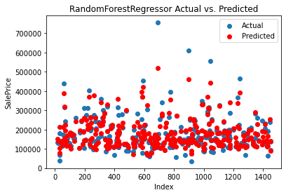
Figure 6. Result of Random Forest.

The random forest regressor demonstrates a similar performance to the SVM model. It achieves an MAE of 18,040.67, indicating a slightly higher average deviation in predictions compared to SVM. The MSE is 950,844,232.54, and the RMSE is 30,835.76, suggesting a lower level of error compared to both linear regression and SVM. The R² score of 0.8760 indicates that approximately 87.60% of the variance in the target variable is explained by the model. The random forest regressor performs well and shows better accuracy and predictive power than linear regression.

4.4. XGBoost

The predicted result compared with the actual is shown in Figure 7.

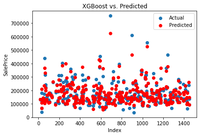
Figure 7. Result of XGBoost.

The XGBoost regression model achieves an MAE of 19,411.23, indicating a higher average deviation in predictions compared to both SVM and random forest. The MSE is 900,813,561.35, and the RMSE is 30,013.56, suggesting a similar level of error as the random forest model. The R² score of 0.8826 indicates that approximately 88.26% of the variance in the target variable is explained by the model. The XGBoost model performs well and shows good accuracy and predictive power, although slightly lower than the random forest regressor.

4.5. Comparison

All the result is shown in Table 4.

Table 4. Results of models.

Figure 8 is the plot that clearly shows the R² of the models, making it convenient to compare the result.

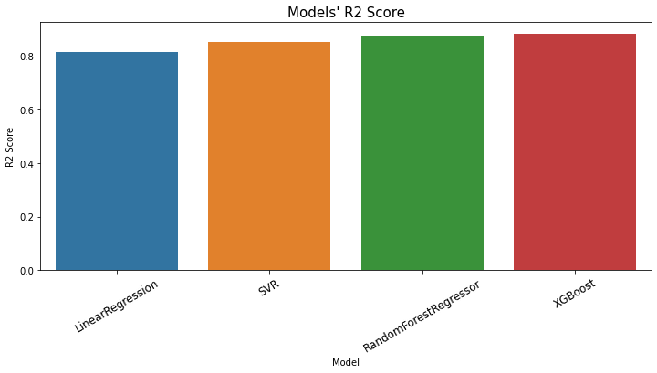
Figure 8. R² of all models.

Among the evaluated models, the XGBoost and random forest regressor models perform the best in terms of accuracy and predictive power, followed closely by the SVM model. Linear regression demonstrates the weakest performance among the four models. However, the choice of the best model depends on the specific requirements and characteristics of the problem at hand, and it’s always recommended to consider other factors such as model complexity and interpretability alongside these evaluation metrics.

5. Discussion

From the research shown above, it can be found that the key factors that may affect the house price are rates for the overall material and finish of the house, original construction date, remodel date, unfinished square feet of basement area, first Floor square feet, above grade living area square feet, full bathrooms above grade, total rooms above grade, size of a garage in car capacity, size of a garage in square feet, condition of sale, identifies the general zoning classification of the sale, type of utilities available, type of dwelling, type of heating, kitchen quality, condition of sale and slope of the property. Also, in this situation, XGBoost has the best performance in predicting the house price. The research can help people learn some methods for predicting house prices.

However, there are some limitations in this research. While Kaggle is a popular platform for accessing and sharing datasets, there are potential disadvantages to using a dataset downloaded from Kaggle and the dataset is one year old.

The dataset may not reflect the current state of the real estate market or the factors influencing house prices. Economic conditions, market trends, and government policies can change significantly within a year, and using outdated data may result in less accurate predictions.

The dataset may have limited coverage in terms of geographical regions, property types, or market segments. Real estate markets can vary greatly across different locations and property categories, and relying on a dataset that lacks diversity may lead to biased or incomplete predictions.

The dataset may contain missing or incomplete data points, which can impact the quality and reliability of the predictions. Missing data can introduce biases or affect the performance of machine learning models if not handled appropriately.

Datasets downloaded from Kaggle may not undergo rigorous quality checks or verification processes. The dataset may contain errors, inconsistencies, or inaccuracies, which can negatively affect the performance of predictive models.

The dataset may not include all relevant features or variables that are known to influence house prices. Missing important predictors can result in suboptimal models and reduced predictive accuracy.

The dataset may lack contextual information or metadata about the variables, making it challenging to interpret and understand the relationships between features and target variables. Understanding the context is crucial for feature engineering, model selection, and decision-making based on predictions.

The dataset may suffer from selection bias or other types of biases that were not adequately addressed during data collection. Biased data can lead to biased predictions and perpetuate inequalities or inaccuracies in the results.

To mitigate these disadvantages, it is important to critically evaluate the dataset’s quality, relevance, and applicability to the current problem at hand. Consider supplementing the dataset with additional data sources, updating the data if possible, and conducting thorough exploratory data analysis to understand the limitations and potential biases in the dataset.

6. Conclusion

The research identifies key factors that may influence house prices, providing valuable insights into the important features to consider when building predictive models. Future research can build upon this foundation by exploring additional features or alternative feature selection techniques to further improve the accuracy and interpretability of the models.

The research compares and evaluates the performance of different regression models, including linear regression, support vector machines (SVM), random forest, and XGBoost. This comparison provides a benchmark for future research, allowing researchers to assess the effectiveness of these models in different contexts or datasets. It also opens avenues for exploring other regression algorithms or ensemble methods for house price prediction.

The research utilizes common evaluation metrics such as mean absolute error (MAE), mean squared error (MSE), root mean squared error (RMSE), and R² score to assess the performance of the models. Future research can consider using these metrics as a standard evaluation framework and explore additional metrics tailored to specific aspects of house price prediction, such as price prediction accuracy within certain tolerance ranges or metrics that capture the economic impact of predictions.

Some suggestions can be helpful in future research. Explore the use of real-time data sources, such as real estate listings, economic indicators, or social media data, to capture the most up-to-date information about the market. This can enhance the accuracy and timeliness of predictions, especially in dynamic and rapidly changing real estate markets. Investigate time series modeling techniques to capture temporal patterns and trends in house prices. Analyze historical price data to identify cyclical or seasonal patterns, assess long-term price trends, and incorporate time-dependent variables that may influence house prices, such as interest rates, inflation rates, or housing market policies. Explore ensemble modeling approaches that combine multiple models or algorithms to improve prediction accuracy and robustness. Techniques such as stacking, boosting, or bagging can be employed to leverage the strengths of different models and mitigate the weaknesses of individual models.

References

[1]. Zhang. J Q, Du. J, “House Price Prediction Model Based on XGBoost and Multiple Machine Learning Methods,” Modern Information Technology vol. 4, no. 10, pp. 15-18, May. 2020.
[2]. Lu. C M, Ma. Z Z, Han. Y, Guo. X Q, “Analysis of House Price Data based on Support Vector Regression”, vol. 43, no. 4, pp. 76-82, Oct. 2021.
[3]. Wei. X, “Analysis of influencing factors of second-hand house price in Nanning City based on random forest”, LIGHT INDUSTRY SCIENCE AND TECHNOLOGY, vol. 37, no. 10, pp. 96-98, Sep. 2021.
[4]. Chen. T Q, Guestrin. C, “XGBoost: A Scalable Tree Boosting System” [J/OL].arXiv: 1603.02754 [cs.LG].(2016-03-09). https://arxiv.org/abs/1603.02754.
[5]. Hu. X W, Ma. C M, Kong. X S, Li. F Y, “Shenzhen second-hand housing price forecast based on XGBoost”, Journal of Qufu Normal University, vol. 48, no. 1, pp. 57-65, Jan. 2022.
[6]. Zhang. Y Z, Jia. L X, “SVR house price forecasting model based on grid optimization -- Taking Zhengzhou City as an example”, vol. 32, no. 8, pp. 1659-1663, Aug. 2014.
[7]. Zhong. A N, Da. X, Yu. J M, “Geographical perspective of housing prices in Shenzhen and its influencing factors -- Based on random forest model”, Urban Geotechnical Investigation & Surveying, no.2, pp.66-70, Apr. 2022.
Cite this article
Chuhan,N. (2024). House price prediction based on different models of machine learning. Applied and Computational Engineering,49,47-57.
Data availability
The datasets used and/or analyzed during the current study will be available from the authors upon reasonable request.
Disclaimer/Publisher's Note
The statements, opinions and data contained in all publications are solely those of the individual author(s) and contributor(s) and not of EWA Publishing and/or the editor(s). EWA Publishing and/or the editor(s) disclaim responsibility for any injury to people or property resulting from any ideas, methods, instructions or products referred to in the content.
About volume
Volume title: Proceedings of the 4th International Conference on Signal Processing and Machine Learning
© 2024 by the author(s). Licensee EWA Publishing, Oxford, UK. This article is an open access article distributed under the terms and
conditions of the Creative Commons Attribution (CC BY) license. Authors who
publish this series agree to the following terms:
1. Authors retain copyright and grant the series right of first publication with the work simultaneously licensed under a Creative Commons
Attribution License that allows others to share the work with an acknowledgment of the work's authorship and initial publication in this
series.
2. Authors are able to enter into separate, additional contractual arrangements for the non-exclusive distribution of the series's published
version of the work (e.g., post it to an institutional repository or publish it in a book), with an acknowledgment of its initial
publication in this series.
3. Authors are permitted and encouraged to post their work online (e.g., in institutional repositories or on their website) prior to and
during the submission process, as it can lead to productive exchanges, as well as earlier and greater citation of published work (See
Open access policy for details).