1. Introduction

Tabular data is an essential foundation across diverse fields, prominently in critical domains like healthcare, factory settings, advertising, and finance. Its inherent structure streamlines various benefits, such as the efficient storage, retrieval, and analysis of multifaceted information. Often employed in regression and classification tasks, tabular data predicts categorical or numerical outcomes based on data rows. This seemingly straightforward process can yield valuable and critical insights for professionals in various sectors, shaping informed decisions.

While for classification and regression tasks involving tabular data, the landscape has been predominantly shaped by models rooted in gradient tree boosting techniques since 2016. This dominance primarily stems from their robustness and efficient training times. Exemplified by well-known implementations like XGBoost, LightGBM, and CatBoost, these models, derived from the gradient boosting methodology, form a pivotal aspect of the machine learning field [1-4]. In machine learning competitions, gradient boosting tree models are particularly prevalent due to their capability to achieve exceptional performance when the hyper parameters are properly tuned.

Another facet of machine learning consists of those traditional algorithms, excelling in their simplicity, speed, and resource efficiency. Notable examples include Logistic Regression, Support Vector Machines (SVM), and k-nearest neighbours. excels at its simplicity, speed. They are frequently employed in sectors such as manufacturing, healthcare, and settings where prediction accuracy is not the goal, but the prediction speed is of paramount importance and computational resources are valued assets.

As the tasks surrounding tabular data is dominate by the traditional and gradient boosting tree machine learning algorithms, the realm of deep learning has striven to bridge the gap in performance for tasks around tabular data, concurrently. To begin with, the Multilayer Perceptron (MLP) model was served as a baseline. Then, various deep learning architectures tailored to tabular data have been formulated, novel models have drawn inspiration from diverse fields; for instance, the adoption of ResNet-like architectures from computer vision and the Transformer architectures from natural language processing [5, 6].

In this paper, we introduce a model that attains prediction accuracy comparable to boosting tree algorithms while maintaining feature interpretability. Achieving this synergy involves encoding continuous features, embedding categorical names, and their respective features. These processed features are then directed injected into a modified Transformer module for prediction. Our adapted Transformer module is meticulously designed to cater to the nuances of tabular data. Given tabular data’s inherent sparsity and the presence of negative values, specific modifications have been implemented. Also, this customized Transformer module features a solitary layer of encoder and decoder. Moreover, the combination of ReLU and layer normalization layers is replaced with an SELU activation layer, effectively preserving the latent information [7].

Furthermore, the specially crafted embedding layer serves the dual purpose of encoding feature names and category names, thereby revealing the intricate interconnections that exist between these categories and features. With the growing emphasis on safeguarding the privacy of personal and business data, approaches of withholding the disclosure of actual feature or category names and replacing them with pseudo-labelled character representations are being applied, as demonstrated in the recent Kaggle ICR competition. The interpretability provided by the embedding layer not only addresses this challenge of anonymity but also contributes to a more thorough comprehension of the intricate relationships between features and categories within specialized datasets, thereby enhancing their overall interpretability.

Finally, in literature review section, related papers are researched and discussed. In the model section, the structure and design of model has been explained. In experiment section, experiment on various datasets is being conducted and the result of our model are being compared to various existing models. In Feature interpretability section, the unique property of our model that allows feature and category interpretability is introduced. Finally, in conclusion section, the result and conclusion of this paper is presented.

2. Literature Review

The primary attention for related paper resides on the models which originated from the Transformer architecture, as it serves as the foundational architecture underlying our work.

Originating as a solution for NLP translation tasks, the Transformer’s core structure encompasses encoder and decoder layers comprising self-attention mechanisms and feedforward neural networks (FFNNs). After the introduction of Transformer, it quickly gains it’s popularity, and the swift proliferation of the Transformer’s popularity in the NLP domain has permeated the broader landscape of deep learning. Notably, computer vision tasks have given rise to variations of Transformer structure, such as the Vision Transformer (ViT) [8]. In alignment with this trend, the field of tabular data analysis has witnessed the emergence of various adaptations of the Transformer.

When Transformer first emerges, model with simple adaptation that only involves modification of input data that allows the input data to be fed into transformer architecture is introduced. The FT-Transformer employs a straightforward yet effective approach [9]. It starts by tokenizing and embedding the categorical features. These embeddings are then combined with the continuous features, which have been processed through a dense layer. This approach enables smooth integration of input features into the Transformer architecture. On the other hand, the Tab-Transformer adopts an approach reminiscent of wide and deep models [10]. It utilizes embeddings to process categorical features, which are subsequently fed into a Transformer layer. At the final dense layer, these embedded representations are combined with the continuous features to form a prediction. These adaptations represent instances of simplistic yet impactful integration of the Transformer model within the tabular data context.

Notably, a subset of models further augments the fundamental Transformer architecture, yielding considerable enhancements in tabular data tasks. For instance, the SAINT model incorporates self-attention mechanisms from Transformers while introducing inter-sample attention, effectively capturing row-wise relationships and used neighbour-based classification for final prediction [11]. ExcelFormer amalgamates Transformer attention mechanisms with FFNNs, proposing AiuM and DiaM modules that facilitate feature representation updates and interactions [12]. TransTab, which shares its lineage with the Transformer architecture, accommodates variable column tables, thus accommodating pre training and transfer learning [13]. Finally, TabPFN, gaining traction in recent Kaggle competitions, harnesses the power of synthetic data and prior data fitting to pre train Transformer-like models, showcasing prowess particularly on small datasets [14].

While the aforementioned models manifest commendable utility, our research endeavours unveil yet another innovative adaptation of the Transformer model tailored to tasks in the tabular domain. Our model is meticulously crafted to address the intricacies and challenges inherent in this context. By modifying the input features to a more favoured representation and feeding it into the modified transformer architecture, where ReLU and layer norm are replaced with SELU activation, for better handling of tabular data.

3. The Model

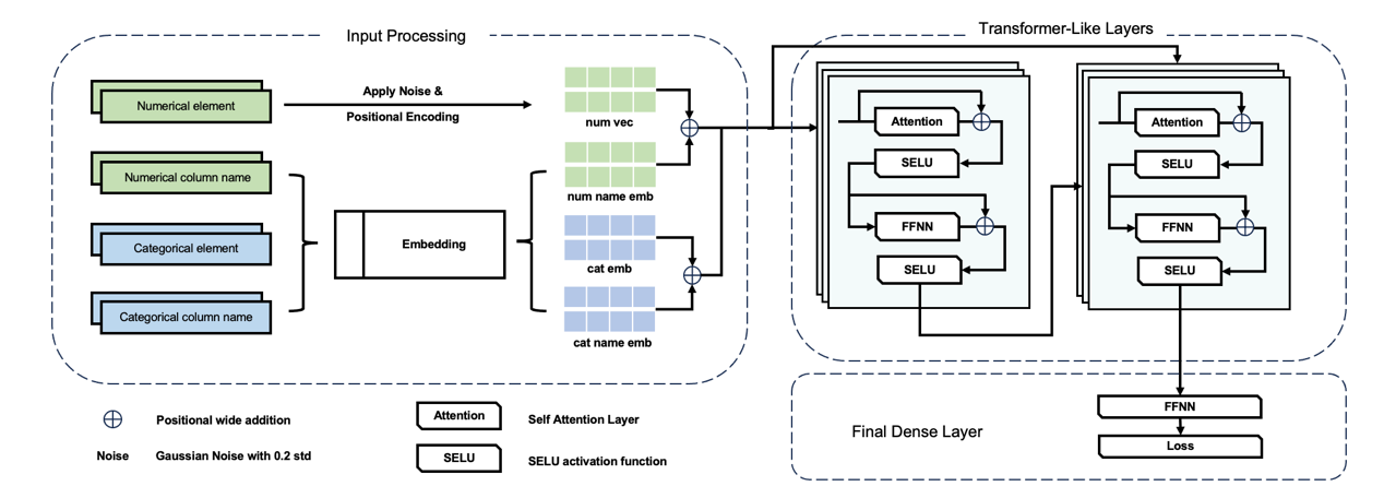
The model is constructed upon the Transformer architecture, and we have adapted this architecture to make it more suitable for addressing classification and regression problems involving tabular data. The overall model architecture is structured as follows: (1) Input processing layers, (2) Transformer-like layers, and (3) Dense layer. A detailed model architecture is shown in Figure 1.

3.1. Input Processing Layers

The first layer before the transformer like structures are the input processing layer. Our model treats any tabular data as decomposition of two elements: categorical element and numerical element. The separation of categorical element and numerical element is driven by its inherent differences. The numerical element encapsulates a continuous range of values, while the categorical element is discrete in natural and lack of mathematical meanings. Additionally, in this paper, categorical elements undergo a direct tokenization and processing through an embedding layer, which is similar to natural language processing tasks, where a unique vector dimension of 64 has been trained to represent each category. In contrast, to align the numerical element to the categorical vector dimension of 64, a modified positional encoding is used, wherein the numerical value itself is adopted as the positional parameter. This approach ensures that each encoded value preserves the same numerical meaning from the input, while simultaneously exhibiting variations across different instances.

3.1.1. Categorical elements. A categorical element can be categorical features, binary features, and column names. An embedding matrix is created with size of categorical elements \( × \) 64. Each categorical element is tokenized and matched to a corresponding row of the embedding matrix to generate a categorical feature embedding vector of size 64.

3.1.2. Numerical elements. The numerical element is any continuous features. A Gaussian noise with standard deviation of 0.2 is first been applied to each numerical element mimicking noise in the datasets and provide more augmentation, so that the model is more robust. Then, to allow continuous features match the shape of categorical feature embedding, the disturbed numerical element has been feed to positional encoding. Since numerical element itself have an underlying aspect of position and we need to expand the numerical element to the same shape of categorical feature embedding, with each position still holds the information of the original data but varies for different position of the vector. The modified positional encoding is as follows:

\( Pe(value,2i)=Sin(\frac{value}{{1000^{\frac{2i}{{d_{model}}}}}}) and Pe(value,2i+1)=Sin(\frac{value}{{1000^{\frac{2i+ 1}{{d_{model}}}}}}) \) (1)

Finally, the embedded categorical column names and numerical column names are being added to the corresponding categorical or numerical vectors. The categorical or numerical vectors are concatenated to form the final input to the transformer-like layers.

3.2. Transformer-like Layers

To tailor the Transformer architecture to the characteristics of Tabular data, several modifications are applied to the architecture.

3.2.1. Transformers The original implementation of Transformer [13] consists of an encoder and decoder, each composed of several identical layers. Each layer consists of a multi-head self-attention layer followed by a feed-forward layer. Additionally, layer normalization and residual connections are used to stabilize training.

Self-attention is a mechanism in the Transformer architecture that enables each position in a sequence to attend to other positions, capturing dependencies between different elements in the sequence. Specifically, a self-attention layer consists of three components: Key \( K ∈{R^{m ×k}} \) , Query \( Q∈{R^{m×k}} \) , and Value \( V∈{R^{m×v}} \) . Each component is being applied to the input. Query and Key are multiplied to produce attention scores, which are used to compute a weighted sum of Values. Mathematically, for a sequence of input vectors X, the self-attention operation can be expressed as:

\( Attention(Q,K,V)=softmax(\frac{Q{K^{T}}}{{({d_{k}})^{\frac{1}{2}}}}) \) \( V \) (2)

Here, Q, K, and V are the transformed Query, Key, and Value matrices, and \( {d_{k}} \) is the dimension of the Key vectors. The softmax function normalizes the attention scores, determining how much each position contributes to the final output.

In practice, when we implement this structure on tabular data, the attention between features can then be captured and applied to the input features to determine the final classification target.

To tailor the Transformer architecture to the characteristics of Tabular data, this paper has embraced the principle of Occam’s Razor, advocating for minimal unnecessary multiplication of entities. As a result, we have streamlined the Transformer’s architecture to have only one encoder and one decoder layer. Furthermore, we have excluded the masked layer from the multi-head attention within the decoder layer. While this masked layer is crucial for preventing the model from accessing future information in Natural Language Processing (NLP) tasks, its absence is justified for Tabular data, where there’s no inherent ordering. Also, in the context of training with tabular data, the presence of masked layer inadvertently restricts preceding data from accessing the subsequent data. Consequently, earlier data receive fewer contextual information, leading to potentially compromised learning outcomes. Hence, the masked layer is removed in the decoder module. Lastly, the combinations of ReLU and layer normalization have been replaced with a SELU activation layer.

3.2.2. SELU Here, we present the rationale behind the decision to substitute the combination of normalization layer and ReLU activation with SELU activation function in our proposed neural network architecture. The substitution is motivated by two key reasons.

• Addressing the “Dying ReLU” problem

The Rectified Linear Unit (ReLU) activation function, mathematically defined as

\( f(x)=max{(0,x)} \) \( . \) (3)

is commonly used due to its simplicity and effectiveness in many machine learning tasks. However, ReLU suffers from the “Dying ReLU” problem, where the problem arises when certain neurons become inactive, consistently producing zero outputs. Given that tabular data inherently differs from computer vision (CV) and natural language processing (NLP) tasks, where ReLU has found widespread adoption, tabular data often contains a substantial number of negative values. The abundance of negative values will inevitably worsen the dying ReLU problem.

Additionally, the architecture proposed, condensed to a single layer of encoder and decoder, is particularly susceptible to the Dying ReLU problem, since there exists less neurons. The excessive presence of negative values in tabular data, coupled with the reduced model depth, would lead to a significant loss of latent information during training. To prevent this issue and retain the valuable information present in negative values, we opted to eliminate the use of ReLU activations.

• Leveraging SELU for Self-Normalization:

The SELU activation function (Scaled Exponential Linear Units) are activation function that induces self-normalization. Mathematically expressed as:

\( f(x)=\begin{cases} \begin{array}{c} λx if x \gt 0 \\ λα({e^{x}}-1)ifx≤0 \end{array} \end{cases} for λ≈1.0507,α≈1.6733 \) \( . \) (4)

SELU activations are equipped with self-normalization property, where the input features are been pushed to zero mean and unit variance. Unlike ReLU, SELU retains both positive and negative values within the data, affectively avoiding the Dying ReLU problem. Furthermore, our decision to utilize SELU activations is bolstered by findings from the original SELU paper, which indicate that SELU outperforms layer normalization used in Transformer architecture and batch normalization, especially when dealing with small perturbations and high variances.

3.3. Final dense layer

The final layer serves as an extractor, retrieving pertinent information from the latent output of the transformer like structure. For Regression tasks, a dense layer is used. For classification tasks, a SoftMax activation is employed after the dense layer, creating an output size that corresponds precisely to the dimensions of the target data.

4. Experiments

4.1. Data

We evaluate our model and baseline models on 2 publicly available classification datasets from UCI repository (Dua and Graff 2017) and Kaggle (Kaggle, Inc 2017). For each dataset, the data is divided into training and testing set, with a split of 80%/20%. The Categorical data is processed with Label encoding. For our model, the categorical column name and continuous column name are being extracted and Label encoded. For our model, the input data are continuous features, label encoded categorical features, continuous column names, and categorical column names. The description of datasets are shown in table 1.

Table 1. Datasets description.

4.2. Model Setup

For each dataset, our model and five baseline model are trained and evaluated. Including Logistic Regression, Random Forest Classifier, MLP Classifier, XGBoost Classifier, and tab transformer. The tab transformer is built with TensorFlow, XGBoost Classifier is obtained from XGBoost package, and all other models are taken from Sklearn module. The hyper parameters are not tuned. For our model, we set a batch size of 64, learning rate of 0.005, with an exponential decay of learning rate with a decay step of 20 and decay rate of 0.9. The model is then trained for 3 epochs for each dataset. Then, each model has been trained and evaluated for 10 times, the subsequent predicted results are being evaluated against the testing target by accuracy rating for classification task. The resulting evaluations are shown in table 2, where the datasets are been mentioned with their abbreviations. The model proposed in this paper is highlighted in grey, and the datasets with the best accuracy score has been coloured with red.

Table 2. Model Performance Comparison

In table 2, when compared with traditional machine learning models, our model consistently outperforms their score. While compared to the similar Neural Network models, our model surpasses the baseline Multi-layer Perception model by a drastic 10%. Comparing to the Tab-transformer model, which is similar to ours’s as it inherent it’s structure from Transformer, our model still consistently outperforms Tab-transformer by an average of 2% for classification tasks. Even when compared with GBDT boosting tree models, such as XGBoost, we only lose merely by 0.2% of accuracy, and the gap is narrowing as the dataset’s size increasing.

4.3. Ablation Experiments

The performance comparison of our model in the cases of with and without SELU activation are presented in table 3.

Table 3. Model Performance Comparison between our model with and without SELU

As anticipated, the incorporation of the SELU activation function effectively tackled the issue of dying ReLU units, thereby retaining a greater amount of latent information and consistently enhancing the final prediction by 0.4%.

In summary, aligning all aspects of the SELU activation layer shows a clear advantage over the combination of layer normalization and ReLU layers, which also further simplified our overall architecture. This strategic choice aims to enhance training effectiveness and information retention, thereby improving the model performance on Tabular data.

5. Feature Interpretability

To visually see the Interpretability of the trained embedding layer, a PCA analysis is applied to the embedding layer of the model trained on the adult capital income dataset. In this analysis, the embedding vectors of dimension 64 are condensed into x and y positions.

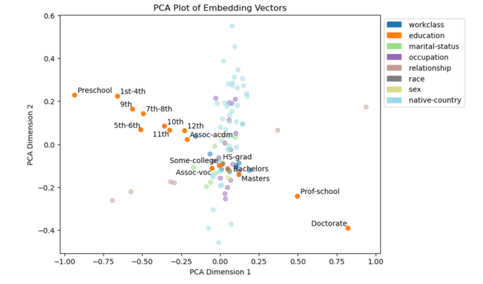
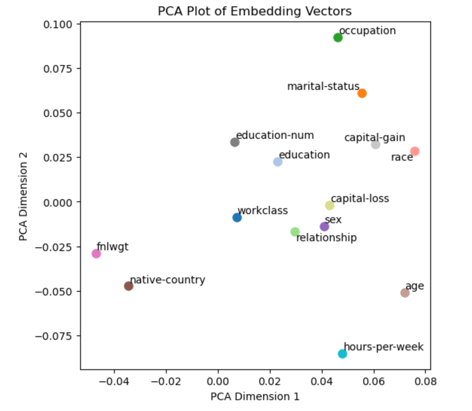
Figure 2 illustrates the PCA analysis of embedding of education categories, revealing a distinct trend between the label position and the level of education. The labels range from preschool, the lowest education level (upper left), to Doctorate, the highest level of education (lower right). Other categories also exist similar relationships between its position and its underlying meaning.

Figure 3 showcases another PCA analysis of embedding of feature names. This analysis provides clear indications of relationships, such as the connection between “education-num” and education, as well as the relationship between “capital gain” and education, race, and marital status.

Indeed, the trained model’s embeddings unveil hidden relationships between features. Even when the feature and category names are concealed, these results can offer the user an intuitive understanding of the datasets.

6. Conclusion

In this paper, a novel model rooting from transformer model adapted specifically to tabular data is presented. The model consists of three parts, input processing part, Transformer-like part, and a final dense layer. For the transformer-like part of the model, all combination of ReLU and layer normalization are being replaced with SELU activation, and the attention mask are being removed to supply the model with more latent information. Additionally, a specially designed input processing layer are used to handle the tabular data. Empirical experiments have consistently demonstrated that the model outperforms traditional machine learning algorithms. Even when compared to similar Transformer-based networks, our model exhibits superior performance. Notably, the model also showcases performance comparable to the state-of-the-art gradient boosting tree models. To further validate our approach, an ablation experiments is conducted. In the experiments, our model consistently outperformed other cases where SELU activation was not used, thus affirming the correctness and effectiveness of our modifications in the Transformer part. Furthermore, one distinctive feature of our model is its ability to offer enhanced interpretability for any given data. The embedding layer within the trained model unveils underlying relationships within categorical features, and continuous and category feature names. This capability proves valuable when categorical and feature names are anonymized or when users are unfamiliar with the domain from which the data originates. Finally, for future work, further adaptation or modification of the model to accommodate small-sized datasets could be explored.

References

[1]. Chen T and Guestrin C 2016 XGBoost: A scalable tree boosting system Proceedings of the 22nd acm sigkdd international conference on knowledge discovery and data mining 785-94
[2]. Ke G, Meng Q, Finley T, Wang T, Chen W, Ma W, Ye Q and Liu TY 2017 Lightgbm: A highly efficient gradient boosting decision tree Advances in neural information processing systems, 30
[3]. Prokhorenkova L, Gusev G, Vorobev A, Dorogush A and Gulin A 2018 CatBoost: unbiased boosting with categorical features Advances in neural information processing systems 31
[4]. Friedman J H 2001 Greedy function approximation: a gradient boosting machine Annals of statistics 1189-232
[5]. He K, Zhang X, Ren S and Sun J 2016 Deep residual learning for image recognition Proceedings of the IEEE conference on computer vision and pattern recognition 770-8.
[6]. Vaswani A, Shazeer N, Parmar N, Uszkoreit J, Jones L, Gomez AN, Kaiser Ł and Polosukhin I 2017 Attention is all you need Advances in neural information processing systems 30
[7]. Klambauer G, Unterthiner T, Mayr A and Hochreiter S 2017 Self-normalizing neural networks Advances in neural information processing systems 30
[8]. Dosovitskiy A, Beyer L, Kolesnikov A, Weissenborn D, Zhai X, Unterthiner T, Dehghani M, Minderer M, Heigold G, Gelly S et al 2020 An image is worth 16x16 words: Transformers for image recognition at scale arXiv preprint arXiv:2010.11929
[9]. Gorishniy Y, Rubachev I, Khrulkov V and Babenko A 2021 Revisiting deep learning models for tabular data Advances in Neural Information Processing Systems 34 18932-43
[10]. Huang X, Khetan A, Cvitkovic M and Karnin Z 2020 Tabtransformer: Tabular data modeling using contextual embeddings arXiv preprint arXiv:2012.06678
[11]. Somepalli G, Goldblum M, Schwarzschild A, Bruss CB and Goldstein T 2021 Saint: Improved neural networks for tabular data via row attention and contrastive pre-training arXiv preprint arXiv:2106.01342
[12]. Chen J, Yan J, Chen DZ and Wu J 2023 ExcelFormer: A Neural Network Surpassing GBDTs on Tabular Data arXiv preprint arXiv:2301.02819
[13]. Wang Z and Sun J 2022 Transtab: Learning transferable tabular transformers across table Advances in Neural Information Processing Systems 35 2902-15
[14]. Hollmann N, Müller S, Eggensperger K and Hutter F 2022 Tabpfn: A transformer that solves small tabular classification problems in a second arXiv preprint arXiv:2207.01848
Cite this article
Mao,Y. (2024). TabTranSELU: A transformer adaptation for solving tabular data. Applied and Computational Engineering,51,81-88.
Data availability
The datasets used and/or analyzed during the current study will be available from the authors upon reasonable request.
Disclaimer/Publisher's Note
The statements, opinions and data contained in all publications are solely those of the individual author(s) and contributor(s) and not of EWA Publishing and/or the editor(s). EWA Publishing and/or the editor(s) disclaim responsibility for any injury to people or property resulting from any ideas, methods, instructions or products referred to in the content.
About volume
Volume title: Proceedings of the 4th International Conference on Signal Processing and Machine Learning
© 2024 by the author(s). Licensee EWA Publishing, Oxford, UK. This article is an open access article distributed under the terms and
conditions of the Creative Commons Attribution (CC BY) license. Authors who
publish this series agree to the following terms:
1. Authors retain copyright and grant the series right of first publication with the work simultaneously licensed under a Creative Commons
Attribution License that allows others to share the work with an acknowledgment of the work's authorship and initial publication in this
series.
2. Authors are able to enter into separate, additional contractual arrangements for the non-exclusive distribution of the series's published
version of the work (e.g., post it to an institutional repository or publish it in a book), with an acknowledgment of its initial
publication in this series.
3. Authors are permitted and encouraged to post their work online (e.g., in institutional repositories or on their website) prior to and
during the submission process, as it can lead to productive exchanges, as well as earlier and greater citation of published work (See
Open access policy for details).