1. Introduction

In the realms of science and technology, professionals continuously grapple with optimizing intricate decision-making mechanisms, striving to achieve the delicate equilibrium between exploration and exploitation. This quandary is encapsulated by the Multi-Armed Bandit (MAB) problem, a cornerstone in the domain of sequential decision-making [1]. It’s essential to understand that while the MAB problem finds its roots in the reinforcement learning domain, it exhibits distinct characteristics when juxtaposed against other prevalent methods, such as supervised machine learning.

The research terrain surrounding the MAB problem and its associated algorithms is rich and expansive, with a particular focus on the non-structured discrete variant. As we venture into augmentations like the introduction of adversaries or the correlation between arms, we unearth layers of nuance and intricacy within the MAB problem. These augmentations, while adding complexity, are often indispensable in molding the foundational understanding of the problem to align with real-world scenarios. Venturing into this intricate labyrinth, this investigation delves deep into the continuum-armed iteration of the MAB challenge. The spotlight is cast upon the Lipschitz Bandits and the trailblazing Zooming Algorithm, setting the stage for a comprehensive exploration of the quantum-chemistry dataset, QM9.

2. Problem Formulation and Regret for the Discrete MAB Problem

2.1. Problem Formulation

A player employs an algorithm that offers a selection of \( K \) different choices, known as ‘arms’, to make during a total of \( T \) rounds/turns (known as the horizon). Each round involves the algorithm making a decision on one of these arms to ‘play’ and subsequently observing a reward associated with that particular choice. The overarching objective of the algorithm is to maximise the cumulative reward it obtains throughout the \( T \) rounds.

This study assumes the following about the discrete MAB problem which future sections build upon [2]:

The Partial Information Game: the algorithm possesses knowledge solely of the reward obtained from the very arm it chooses at each round. It does not gain access to the reward information corresponding to the other unchosen arms (full information).

The rewards associated with each arm selection are drawn from probability distributions. For each arm, there exists a distinct reward distribution over the real numbers. Whenever an arm is chosen, the reward observed is sampled independently from the distribution specific to that arm. The algorithm begins with no prior knowledge of these distributions.

The rewards fall within a bounded range. In controlled experiments this is usually restricted to \( [0, 1] \) for simplicity.

2.2. Regret and Expected Regret

The primary concern lies with the mean reward vector denoted as \( μ∈{[0, 1]^{K}} \) where \( μ(a) \) represents the average reward for a particular arm. The way one formally assesses an algorithm’s performance is through the ‘regret’. Use \( {μ^{*}} \) to represent the expected reward of the best arm. Probabilistically speaking the best ‘strategy’ is therefore to play that best arm for all rounds. To measure this against the cumulative reward generated by the algorithm, introduce the concept of regret at round \( T \) :

\( R(T)={μ^{*}}\cdot T-\sum _{t=1}^{T}μ({a_{t}}) \) (1)

Since \( {a_{t}} \) , the arm selected at round \( t \) , yields a value realised through sampling from a random distribution, \( R(t) \) is inherently a random variable. Hence the focus revolves around the ‘expected regret’, often denoted as \( E[R(T)] \) .

3. Continuum-armed Bandits

This section focuses on the continuous-case extension of the MAB problem. In particular the concept of Lipschitz Bandits is introduced. The motivation comes from the intuition that similar initiatives should result in similar rewards. For example, the similarity between two actions can be quantified by the distance between a pair of feature vectors. The mathematics behind metric spaces makes this consistent throughout the action set, thereby allowing the use of similar actions to guarantee similar rewards [3]. To tackle the MAB problem in a Lipschitz context, this study employs what is called a ‘zooming algorithm’ – which is a class of algorithms that share the same philosophy.

In the continuum-armed framework, the ‘action set’ refers to the collection of possible actions (arms) an algorithm can make in a continuous action space.

3.1. Lipschitz Bandits

3.1.1. Definition. Consider an action set denoted as \( X \) , along with an unknown mean reward function \( u:X→[0,1] \) subject to the condition:

\( |Μ(x)-μ(y)|≤δ(x,y), for all x,y∈X, where δ(x,y) \gt 0 \) (2)

Now define \( D(x,y) \) as the infimum of the sum \( \sum _{t}δ({x_{t}},{x_{t+1}}) \) over all finite such paths \( (x={x_{0}},{x_{1}},…,{x_{k}}=y) \) within the action set \( X \) . This defines a metric.

Consequently, express the Lipschitz inequality as:

\( |Μ(x)-μ(y)|≤D(x,y), for all x,y∈X \) (3)

Here, \( μ \) represents a Lipschitz function with a Lipschitz constant of \( 1 \) concerning the metric space \( (X,D) \) . Going forwards this study will denote an instance of the Lipschitz bandit problem as \( (X,D,μ) \) [4].

Without loss of generality, one may assume the diameter of \( (X,D) \) to be at most \( 1 \) since for any bounded non-negative reward interval it is possible to transform it into the \( [0,1] \) interval.

3.1.2. Definition. In the context of the Lipschitz bandits problem, introduce the term ‘discretisation’ for any predetermined subset \( S \) within the action set \( X \) . Such subset \( S \) may be discrete or uniform and is called a discretisation of \( X \) .

In practice, it is a common practice to utilise the discretisation as an approximation for the action set. Such approximation comes with a discretisation error.

3.1.3. Definition. Define \( {μ^{*}}(S) \) as the highest expected (optimal) reward in \( S \) so that \( {μ^{*}}(S)={sup_{x∈S}}μ(x) \) . It follows that the discretisation error \( DE(S) \) (with respect to \( X \) ) is:

\( DE(S)={μ^{*}}(X)-{μ^{*}}(S) \) (4)

It is important to note that, from the definition, the discretisation error is inherently bounded by the smallest distance between any point in \( S \) to the optimal arm \( {x^{*}} \) (from 3.1.1):

\( DE(S)≤D(S,{x^{*}})≔\underset{x∈S}{min}{D}(x,{x^{*}}) \) (5)

3.2. Zooming Algorithm

3.2.1. Definition. One can consider arms chosen in the discretisation subset \( S \) as probes strategically positioned within the metric space. The objective of an algorithm is to gradually approximate the mean rewards and dynamically adjust the placement of these probes. Such adaptation ensures a greater concentration of probes in regions of the metric space deemed more ‘promising’. This is called adaptive discretisation.

Adaptive discretisation is implemented via the Zooming Algorithm. The algorithm actively maintains a set \( S⊂X \) of active arms. During each round, a selection of arms may be activated based on a predefined activation rule. Subsequently, the algorithm chooses one active arm to play based on a selection rule.

It is worth noting that an active arm stays activated. There is no deactivation rule unless stated otherwise.

3.2.2. Confidence Ball. Assume at round \( t \) an arm \( x \) is active. Define \( {n_{t}}(x) \) to be the number of times \( x \) was played up to round \( t \) . Then let \( {μ_{t}}(x) \) be the sample mean reward of arm \( x \) at round \( t \) , and \( {μ_{t}}(x)=0 \) when \( {n_{t}}(x)=0 \) .

3.2.3. Definition. Given the value of the horizon \( T \) the confidence radius of \( x \) at round \( t \) is:

\( {r_{t}}(x)=\sqrt[]{\frac{2logT}{1+{n_{t}}(x)}} \) (6)

This is similar to the UCB1 (Upper Confidence Bound) index used for discrete bandits. The confidence radius ensures that, with high probability, it bounds the difference between the sample mean reward \( {μ_{t}}(x) \) and arm \( x \) ’s true excepted reward for all arms \( x \) and round \( t \) :

\( |{μ_{t}}(x)-μ(x)|≤{r_{t}}(x) \) (7)

3.2.4. Definition. At round \( t \) , the confidence ball around arm \( x \) is defined as follows:

\( B(x,{r_{t}}(x))=\lbrace \hat{x}∈X:D(x,\hat{x})≤{r_{t}}(x)\rbrace \) (8)

The information provided by the sample observed rewards from arm \( x \) up to round \( t \) enables one to estimate the value of \( μ(x) \) up to an accuracy of \( ±{r_{t}}(x) \) (from 3.2.3). There is also not enough information to distinguish arm \( x \) from other arms within the confidence ball.

3.2.5. Activation Rule. Say that if arm \( x \) is contained in some active arm’s confidence ball, it is ‘covered’. Take an inactive arm \( y \) at round \( t \) which is covered in arm \( x \) ’s confidence ball such that \( D(x,y)≪{r_{t}}(x) \) . There is no need to activate arm \( y \) because there is insufficient information (samples of \( x \) ) to distinguish \( y \) from \( x \) . Still, the following must be maintained throughout: at any round \( t \) , all arms are covered.

Note that an active arm is trivially covered in its own confidence ball, and since the confidence radius of any arm that is being activated for the first time is defined to be greater than \( 1 \) , all arms are covered by that particular arm. The confidence radii decrease as more information is gathered, so an arm \( y \) can become uncovered after play at round \( t \) . Any uncovered arm is then to be activated.

To summarise the steps, one can think of the Zooming Algorithm as self-adjusting: it zooms in on part of the metric iff the arms within are played often iff these arms have promising returns (large sample mean rewards). This is essentially the exploration-exploitation trade-off adapted in a continuous setting.

3.2.6. Selection Rule. To select an arm to play, it must be active at round \( t \) with the largest confidence index value defined as:

\( {CI_{t}}(x)={μ_{t}}(x)+2{r_{t}}(x) \) (9)

For \( C{I_{t}}(x) \) to be large, it is necessary that either \( {μ_{t}}(x) \) is large i.e. arm \( x \) is likely a good arm, or \( {r_{t}}(x) \) is large i.e. there is not enough information on arm \( x \) and the algorithm will more likely actively explore this arm.

3.2.7. Algorithm Overview

Table 1. Algorithm flow.

4. Application to QM9

The QM9 dataset provides detailed information on 134,000 stable small organic molecules [5], covering essential properties like geometry, energy, electronic structure, and thermodynamics [6]. It has gained prominence in the field of computational chemistry due to its exceptional utility in exploring the chemical compound space. As the scientific field move on to using computational methods to design new drugs and materials with desired properties, understanding and navigating this space is of paramount importance. This dataset can be adapted to create, train and assess models based on inductive statistical data analysis [7]. Furthermore, it has the potential to aid in the exploration of previously undiscovered patterns, the identification of relationships between molecular structures and properties, and the design of new molecular materials.

The quest to design novel molecules with tailored properties remains a rather challenging topic. High-throughput screening approaches, although powerful, assume that modelling techniques apply uniformly across chemical space [8]. Due to the exponential growth of the chemical space this assumption often falls short. This limitation underscores the need for innovative strategies to navigate and explore this vast territory.

One such approach involves the application of MAB with adaptive discretisation introduced in earlier sections. In the context of QM9, the MAB implementations in this study can serve as a benchmark for future reinforcement learning studies to pave the way for the development of novel methods. This study aims to systematically navigate the chemical space and adaptively select desirable molecular configurations to maximise the understanding of structure-property relationships.

4.1. Problem Design

The data simulations in this study utilises a subset of the QM9 dataset that contains 6095 isomers of C7O2H10 with orbital energies calculated at G4MP2 level [9]. The Zooming Algorithm will utilise molecular structural similarity information for adaptive discretisation to optimise ‘reward’ over time. The ‘reward’ here is chosen to be the energy gap between LUMO and HOMO (highest/lowest occupied molecular orbital) normalised to \( [0, 1] \) . To make the arm pulling a stochastic process a zero-mean Gaussian noise is added to the gap value, so a noisy value is observed each time an arm is chosen. A key assumption made in the simulations is that the horizon i.e. total number of rounds to play is predetermined and in fact, less than the total number of arms available. Discrete MAB algorithms that assume no discretisation in this case are therefore not applicable. Even if the horizon is extended to accommodate methods such as UCB1 and Thompson Sampling with no discretisation, the optimisation process would still be massively inefficient.

Working with limited resources is a very prevalent issue in practice so this study is interested in gauging whether the Zooming Algorithm can effectively utilise the proposed similarity information to make decisions that optimise reward over a short period of time. This is to be combined with a brief investigation on the algorithm’s ability to adapt to different levels of noise.

4.2. Ultrafast Shape Recognition (USR)

Ultrafast Shape Recognition (USR) is a very popular molecular shape similarity method based on atomic distances [10]. It was developed to address alignment and speed challenges encountered with other shape similarity techniques, therefore suitable for this investigation. USR computes to the distribution of atomic distances from four reference points: the molecular centroid, the nearest atom to the centroid, the farthest atom from the centroid and the atom furthest from the last one. Then it calculates the first three statistical moments for each of these distributions. As a result, each molecule is represented by a 12-value descriptor vector that captures its three-dimensional shape. The assess the similarity between the shapes of two molecules, USR uses the inverse of the Manhattan distances computed from the descriptor vectors [11]. Note the distance is equivalent to the dissimilarity between molecules.

\( {S_{ij}}=\frac{1}{1+\frac{1}{12}\sum _{12}^{k=1}|M_{k}^{i}-M_{k}^{j}|} \) (10)

Figure 1 and Figure 2 reveal some information on the distribution of USR similarities within the data (~6000 isomers). There appears to be no inherent issue/anomalies and the dataset is not structured according to similarity by default.

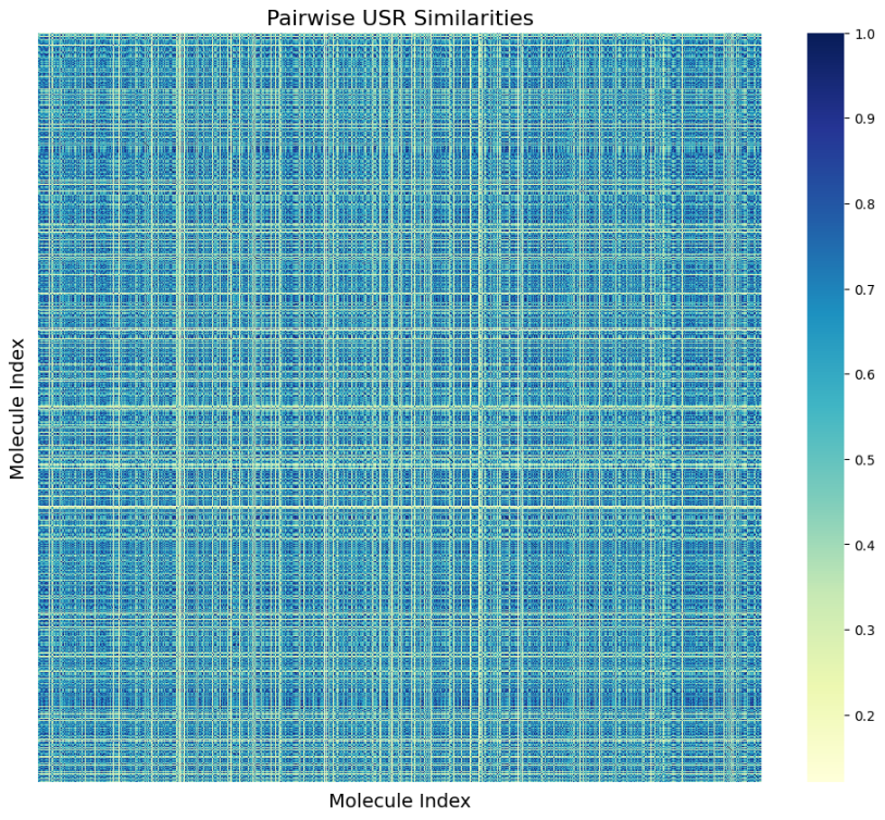
Figure 1. USR Similarity Matrix (Photo/Picture credit: Original).

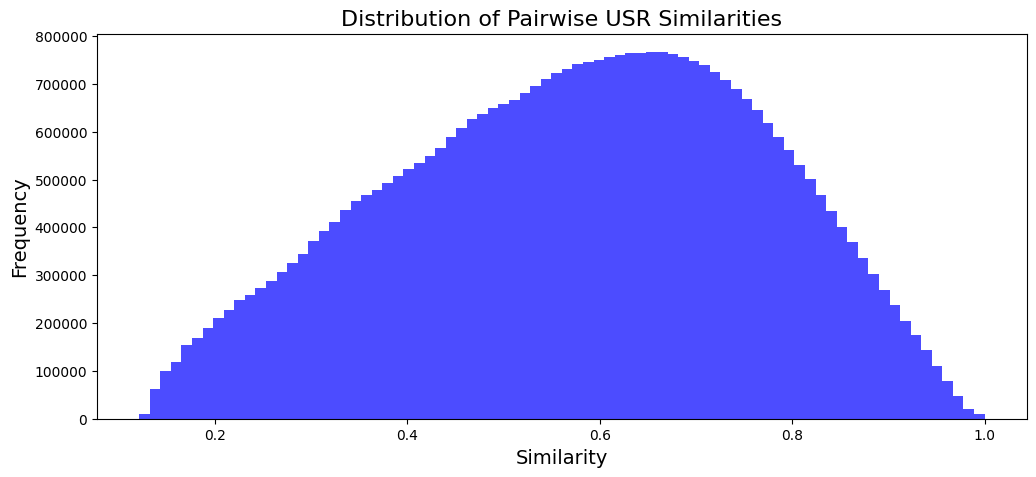
Figure 2. USR Similarity Distribution (Photo/Picture credit: Original).

4.3. Confidence Radius Scaling

The simulations that follow will incorporate a scaling factor to the confidence radius detailed earlier:

\( {r_{t}}(x)=\sqrt[]{(\frac{2logT}{(1+{n_{t}}(x))})}×s if {n_{t}}(x) \gt 0 \) (11)

Where \( s∈[0,1] \) acts as a hyperparameter that adjusts the level of confidence for the Zooming Algorithm and consequently how aggressively it zooms in with the same amount of information gained on the arms (expect the scaling factor to have an effect on the number of active arms). The full distribution of the arm rewards i.e. normalised gap values is shown in Figure 3. By definition the optimal reward value is \( 1 \) and upon inspection the gap values seem to form two peaks at different values. An algorithm will need to at least consistently identify arms around the higher-valued peak that leads to smaller regret buildups and outperform random guessing (equivalent to systematically ‘exploring’ in this unordered dataset). With limited rounds to play, it is harder to identify arms closer to the most optimal one.

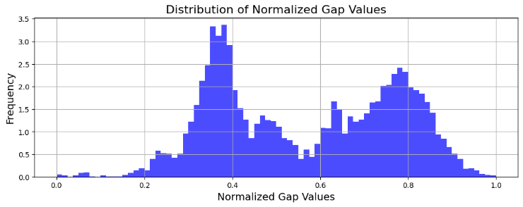
Figure 3. Distribution of Gap Values (Photo/Picture credit: Original).

4.4. Results and Regret Analysis

For the horizon \( T=5000 \) , the following plots of cumulative regret curves use the mean values of \( 100 \) simulations and the \( ~95\% \) confidence regions by taking \( ±2σ \) at each timestep. The Gaussian noise variance values are \( 0.05 \) (moderate, less than \( 10\% \) perturbation on average), \( 0.1 \) (high) and \( 0.2 \) (higher, such that observed rewards from arms of different peaks in Figure 3 are at times indistinguishable). In practice, when working with chemical datasets one can often be able to assume very reliable and accurate approximations of molecular energies. This is the case with this dataset which is calculated at G4MP2 level for less than 10 non-hydrogen atoms [12], although the simulations ran would still try to push the algorithms to make sure they do act predictably and do not break down when faced with more noise than expected in practice. The scaling factors chosen for visualisation are \( 0.04, 0.08, 0.1, 0.5, 0.9, 1 \) . Note that the initial confidence radii of arms that contain no information is not affected by the scaling, so that the assumptions in 3.2.5 still hold. A random arm is chosen at the start of each simulation.

See Figure 4, Figure 5, and Figure 6 for the simulation results.

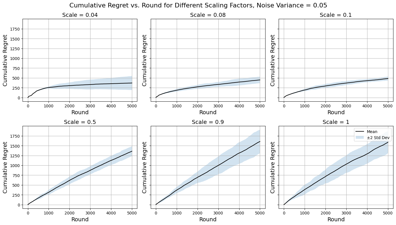
Figure 4. Regret Curves for \( {σ^{2}}=0.05 \) (Photo/Picture credit: Original).

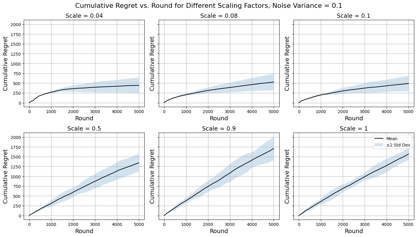
Figure 5. Regret Curves for \( {σ^{2}}=0.1 \) (Photo/Picture credit: Original).

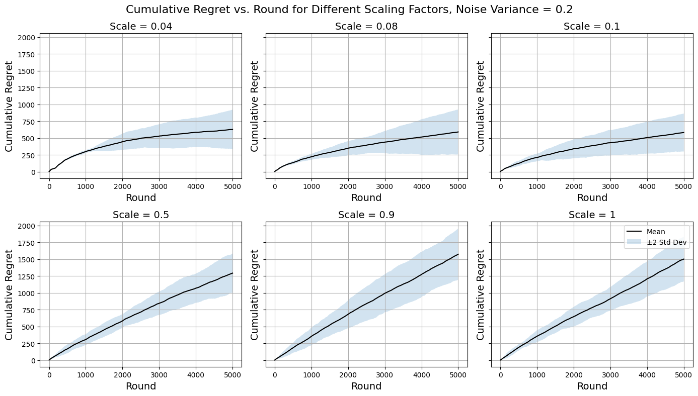
Figure 6. Regret Curves for \( {σ^{2}}=0.2 \) (Photo/Picture credit: Original).

Changing the value of the scaling factor is significant to the overall performance of the Zooming Algorithm on the dataset, therefore it is necessary to tune the value of the scaling factor as a hyperparameter in future studies to optimise the outcome.

Examining the regret curves for \( {σ^{2}}=0.05 \) in Figure 4 reveals that the algorithm tends to do worse for higher scaling factors. For larger values of the scaling factor, arms become uncovered very infrequently therefore the algorithm is not fully capable of making use of the abundancy of the information available and instead limits its vision on too few arms. This does also cause the inconsistency issue as illustrated by the enlarged confidence regions. Nevertheless, they are extremely quick to compute for that reason, and the algorithm still makes use of the similarity information to an extent that it outperforms a naïve purely explorative approach from the get-go. There are signs of the regret curves flattening, so one could speculate that for a longer period of time beyond the current horizon the algorithms using higher scaling factors could be favourable since they eventually will optimise. In the case that computational resource restraint is more significant than the restraint on the horizon (the latter being one of this study’s simulation assumption), they are possibly more favourable. The interest of fine-tuning the scaling factor mainly lies in the smaller values around \( 0.1 \) . Here the regret curves are much more desirable as the algorithms quickly adjust to playing the better arms and optimise the decision-making process over time. The adaptive discretisation here encourages activating more arms for exploration at the expense of higher computational costs and is more effective at using similarity information to identify optimal arms compared to using higher scaling factors. The decreasing regret gradient over rounds is another evidence that supports this. The trends suggest possible logarithmic asymptotic behaviour, which fits with the theoretical results from Introduction to multi-armed bandits (Slivkins, A., 2022) under the regret analysis and upper bound of Lipschitz bandits. It is worth noting that setting the scaling factor too low drives the algorithm towards random exploration which is inconsistent and heavily computationally costly. It is important to take into account all the abovementioned points when designing an implementation and the ‘optimal’ hyperparameter value is totally dependent on the context of the problem one has at hand.

Moving on to performances on noisier data (Figure 5, Figure 6) the general trends across scaling factors to be about the same as above as expected since there are no inherent differences that would cause the same reasoning approach to breakdown. The algorithms do on average tend to perform slightly poorer with increased noise, but it is their inconsistency (illustrated by large confidence regions) that increases more significantly even for cases where they perform well. Still there are no signs of major malfunctions and the Zooming Algorithm remains a reasonably robust method to approach the MAB problem designed for this dataset, since the similarity information between arms proved to be enough to overcome the noise added to obscure the true rewards.

4.5. Active Arms and Scaling Factor

It was remarked earlier that changing the scaling factor affects the number of active arms, which is a trade-off between computational efficiency and gathering information on the full set of arms. Table 1 outlines the average number of active arms at the end of the simulations for each noise and scaling factor simulated in 4.4.

Table 2. Average num. of active arms at the end of the simulation.

The active number of arms at end of the simulations show no correlation with the noise introduced to the arms’ rewards. See Figure 7 for the exponential-like behaviour of arm activation as scaling factor changes. Note that the number of active arms is directly proportional to computation cost since a finer discretisation/definition requires more calculations to be done. As shown in Table 2.

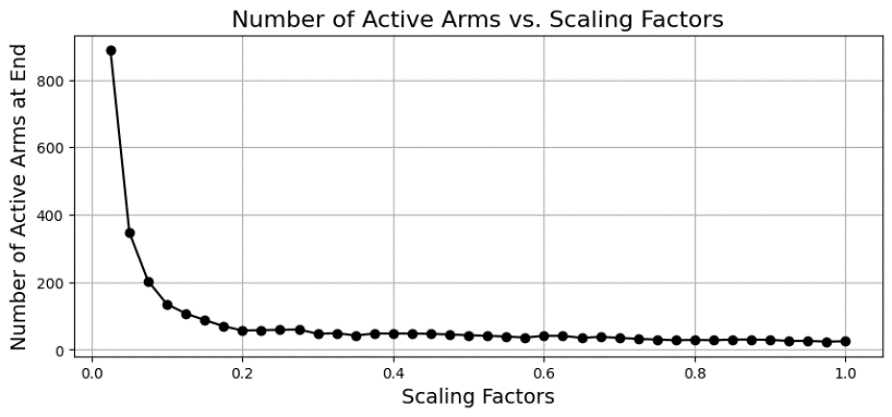
Figure 7. Active arms at end against scaling factors, \( {σ^{2}}=0.05 \) (Photo/Picture credit: Original).

5. Conclusion

In this rigorous computational benchmark study, we tackled the intricate challenge of refining molecular design through the lens of Multi-Armed Bandits (MAB) coupled with adaptive discretisation. We delved into the pioneering concepts of Lipschitz Bandits and the Zooming Algorithm, which provided a dynamic framework to proficiently traverse the vast chemical realm. Our discoveries underscore the prowess of the Ultrafast Shape Recognition (USR) method in gauging molecular similarity. Furthermore, the adept application of the Zooming Algorithm yielded encouraging outcomes, harnessing similarity data to fine-tune molecular blueprints. A pivotal insight emerged regarding the subtle art of modulating a hyperparameter—the scaling factor. This factor was instrumental in orchestrating a harmony between computational prowess and optimal outcomes. It became evident that leaner scaling factors expedited adaptability, resulting in diminished regret, thereby spotlighting the paramountcy of meticulous parameter calibration. It’s worth noting that this exploration shed light on the constraints tied to conventional discrete MAB techniques, especially when operating within constricted resource boundaries—be it rounds or otherwise. Yet, the adaptive discretisation paradigm showcased its merit by sidestepping these very constraints, emerging as a beacon of hope in the quest for molecular design perfection.

This study, while setting a robust platform for future synergistic endeavors straddling mathematics and chemistry, also offers invaluable insights for scholars. They are equipped with a refined understanding of the nuanced equilibrium between computational agility and performance, especially while leveraging the Zooming Algorithm. Furthermore, this exploration paves the way for delving deeper into ancillary avenues, like network and cluster analysis, enhancing the nuances of the reinforcement learning journey. Given the versatility of MAB coupled with adaptive discretisation, the horizon looks promising for surmounting multifaceted optimization quandaries in molecular design.

References

[1]. Mahajan, A., Teneketzis, D. (2008). “Multi-armed bandit problems.” Foundations and Applications of Sensor Management, 2008, 121–151.
[2]. Slivkins, A. (2022). “Introduction to multi-armed bandits.” Available from: https:// arxiv. Org /abs /1904.07272.
[3]. Podimata, C., Slivkins, A. (2021). “Adaptive discretization for adversarial Lipschitz Bandits.” Available from: https://arxiv.org/abs/2006.12367.
[4]. Kleinberg, R., Slivkins, A., Upfal, E. (2019). “Bandits and experts in metric spaces.” Available from: https://arxiv.org/abs/1312.1277.
[5]. Ramakrishnan, R. et al. (2014). “Quantum chemistry structures and properties of 134k molecules.” Sci. Data, 1, 140022.
[6]. Ruddigkeit, L. et al. (2012). “Enumeration of 166 billion organic small molecules in the GDB-17 database.” J. Chem. Inf. Model., 52(11), 2864–2875.
[7]. Rupp M., Tkatchenko A., Müller K. R., von Lilienfeld O. A. (2018). “Fast and accurate modeling of molecular atomization energies with machine learning.” Phys Rev Lett., 108:058301.
[8]. Curtarolo, S. et al. (2013). “The high-throughput highway to computational materials design.” Nature Mater, 12, 191–201.
[9]. Curtiss, L. A., Redfern, P. C., Raghavachari, K. (2007). “Gaussian-4 theory using reduced order perturbation theory.” Journal of Chemical Physics, 127(12), 124105. doi: 10.1063/ 1.2770701.
[10]. Ballester, P. J., Richards, W. G. (2007). “Ultrafast shape recognition to search compound databases for similar molecular shapes.” J. Comput. Chem., 28, 1711–1723. doi: 10.1002/ jcc.20681.
[11]. Kumar, A., Zhang KYJ. (2018). “Advances in the Development of Shape Similarity Methods and Their Application in Drug Discovery.” Front. Chem. 6:315. doi: 10.3389/ fchem. 2018. 00315.
[12]. Dandu, N.K., Assary, R.S., Redfern, P.C., Ward, L., Foster, I., Curtiss, L.A. (2022). “The Journal of Physical Chemistry A, 126(27), 4528-4536.” DOI: 10.1021/acs.jpca.2c01327.
Cite this article
Shi,L. (2024). Optimizing molecular design through Multi-Armed Bandits and adaptive discretization: A computational benchmark investigation. Applied and Computational Engineering,50,69-79.
Data availability
The datasets used and/or analyzed during the current study will be available from the authors upon reasonable request.
Disclaimer/Publisher's Note
The statements, opinions and data contained in all publications are solely those of the individual author(s) and contributor(s) and not of EWA Publishing and/or the editor(s). EWA Publishing and/or the editor(s) disclaim responsibility for any injury to people or property resulting from any ideas, methods, instructions or products referred to in the content.
About volume
Volume title: Proceedings of the 4th International Conference on Signal Processing and Machine Learning
© 2024 by the author(s). Licensee EWA Publishing, Oxford, UK. This article is an open access article distributed under the terms and
conditions of the Creative Commons Attribution (CC BY) license. Authors who
publish this series agree to the following terms:
1. Authors retain copyright and grant the series right of first publication with the work simultaneously licensed under a Creative Commons
Attribution License that allows others to share the work with an acknowledgment of the work's authorship and initial publication in this
series.
2. Authors are able to enter into separate, additional contractual arrangements for the non-exclusive distribution of the series's published
version of the work (e.g., post it to an institutional repository or publish it in a book), with an acknowledgment of its initial
publication in this series.
3. Authors are permitted and encouraged to post their work online (e.g., in institutional repositories or on their website) prior to and
during the submission process, as it can lead to productive exchanges, as well as earlier and greater citation of published work (See
Open access policy for details).