1 Introduction

Interactive image colorization is the process of adding specific colors at any location in a grayscale image to obtain the desired colored image. Grayscale image colorization has found widespread applications in some vision fields, such as medical imaging, cultural heritage preservation, art creation, and video games. Grayscale images are processed to be more realistic and colorful, which is beneficial to improving the performance of downstream computer vision tasks. Traditional colorization methods [1-3] rely on statistical features or mathematical models with higher interpretability, but the results are not ideal. These mathematical models have difficulty processing complex texture and semantic information, so their application on high-resolution images is poor.

Colorization methods based on deep learning learn color change patterns from large-scale color images and can reduce or even eliminate manual intervention. These methods can be further categorized based on whether they require user input of initial colors, resulting in fully automatic image colorization and interactive image colorization.

This paper focuses on interactive image colorization, which, compared to fully automatic colorization, allows users to input initial color points. This integration of model-based approaches with human expertise and artistic intuition enhances the quality and freedom of colorization, thereby assisting professionals in executing more precise and creative colorization. In existing research methods [4-9], to expand the model's receptive field and propagate color cues to distant regions awaiting colorization, a common approach involves the design of heavily stacked Convolutional Neural Networks (CNNs). The color information of large semantic areas is only propagated in deep CNNs, and the transitional connections of color in spatial areas are often ignored. Therefore, ensuring global color consistency has become a difficulty in image colorization, and color changes in complex image scenes often suffer from inconsistent changes. To expand the receptive field of the model and propagate the dependence of color cues to distant areas to be colored, the stacked convolutional neural network (CNN) was abandoned. This article adopts the Transformer architecture that can perform long-distance dependencies. network. By adopting the visual transformer (ViT) architecture [10] to solve this problem, the global receptive field dependence of the self-attention layer is exploited to selectively propagate color cues to distant spatial regions.

However, the Transformer architecture has high computational complexity in image processing and requires a large amount of computing resources and training time. At the same time, the Transformer architecture is highly sensitive to the sample size of the data set. Therefore, this paper introduces a local window self-attention mechanism on top of the ViT architecture to reduce model complexity. Spatial connections between individual local image patches are established. The introduction of the local window self-attention mechanism is mainly to pay attention to the spatial correlation between image blocks and increase the smoothness of colors between image blocks.

For the constraints of inter-block correlation, image blocks are divided into multiple clusters, and self-attention within each cluster is calculated. Furthermore, to capture the correlation of features between blocks, this paper draws on the mathematical models used in traditional image colorization methods and introduces brightness similarity as a criterion for clustering. Thus, connections between spatially distant but still related image patches are established. In order to improve the upsampling effect, we improved the output channel strategy in the layered vision transformer stage to retain more channel information. At the same time, a local stabilization layer is designed before upsampling to reduce artifacts. In the experimental validation section, the interpretability and feasibility of the model are verified and explained. The flowchart of the proposed method is shown in figure 1.

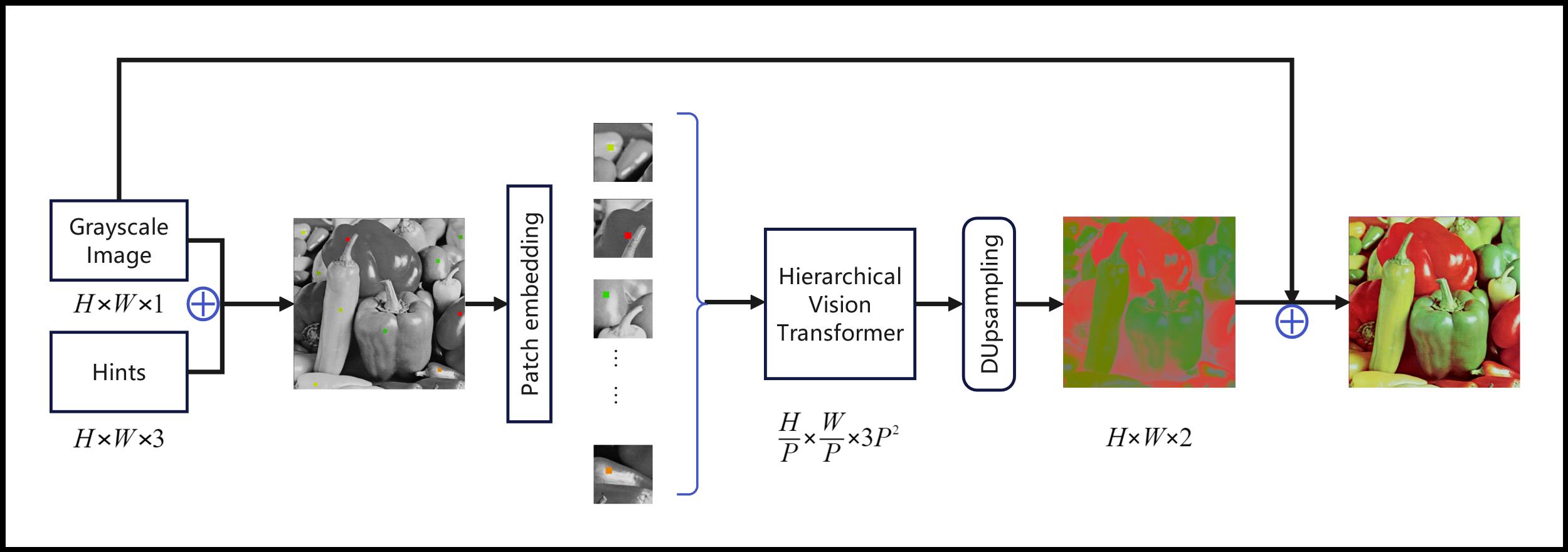Figure 1. Flowchart of the proposed method.

Our contributions are as follows:

1)To address the problem of the high computational complexity of Vision Transformer in colorization, a hierarchical transformer module based on dual local self-attention is proposed.

2)To preserve as much local window information as possible within the hierarchical transformer, improvements are made to the block merging module to increase the color smoothness of the upsampled results.

3)Brightness similarity is introduced as a feature clustering metric for the clustering of critical information. The model's ability to extract local features is enhanced while saving parameters.

2 Related work

2.1 Colorization

Traditional image colorization methods usually rely on manual rules, mathematical models, or statistical methods for image colorization. These can be divided into two categories: color diffusion-based and color transfer-based.

In the field of color diffusion, Levin et al. [1] believe that pixels with similar brightness should have similar color information after colorizing. A weighting method is used to minimize the color difference between each pixel and its neighboring pixels, thereby inferring the color information of neighboring pixels. In the field of color transfer, Welsh et al. [2] first input a color image that is similar to a grayscale image, and then use regional similarity as the basis for pixel matching. This method transfers color information from a color image to a grayscale image to achieve color transfer. Although traditional methods have the advantage of strong interpretability. However, their diffusion functions are difficult to handle complex texture and semantic information, making them difficult to be suitable for large-scale and high-resolution images. Deshpande et al. [4] solved the task of image colorization using a convolutional neural network (CNN) architecture. A relatively simple CNN network is adopted, while the histogram is incorporated into the mean squared error L2 loss function. This method demonstrates the effectiveness of CNN architectures in solving image colorization without the need for reference images or manual interaction. Qin et al. [6] discussed an image colorization method using coding. This method is more efficient, saves memory, and achieves natural shading effects.

Automatic image colorization lacks the flexibility of human-computer interaction. The point interactive colorization model colors the image by specifying colors at different point positions. Because the range of points indicating spatial location is limited to 2x2 to 7x7 pixels, covering only a small portion of the entire image, reasonable results can be obtained with minimal user interaction. Zhang et al. [7] introduced a framework based on user-guided image colorization. Convolutional neural networks (CNN) are used to map sparsely cued grayscale images into real color images with real-time availability. In the study by Su et al. [8], instance-aware shading is used to solve the shading of multiple image objects. Object detection is used to identify individual objects in an image and color them accordingly. The model of Su et al. is not a point interactive colorization model, but an unconditional model. However, its model structure and objective function are the same as the model of Zhang et al., and it can be easily extended to the interactive model. Yin et al. [9] introduced Side Window Filtering (SWF). Window edges or corners are used to align to pixels rather than to the center of the image. This approach improves the edge preservation of color. Yun et al. [11] introduced the ViT framework for point interactive image colorization, but it was limited by the Transformer architecture, which had problems such as large number of parameters and high computational cost. Lee et al. [12] propose a novel A-ColViT architecture to adaptively prune the layers of vision transformer for every input sample. This method flexibly allocates computational resources of input samples, effectively achieving actual acceleration.

2.2 Swin Transformer

Transformer [13] is a network architecture based on the self-attention mechanism, originally designed for the field of natural language processing (NLP). Known as the Vision Transformer (ViT) model, it has demonstrated significant advantages in tasks such as image classification. In ViT, the image is divided into blocks of a series of "patches", while a linear embedding layer is used to convert the patches into vector representations, and then these patches are fed as input elements to the encoder. The multi-head self-attention (MSA) module is used to calculate the relationship between different patches. However, images have higher pixel resolution, which makes training of MSA of patches require a higher sample size.

To solve the problem of a large number of parameters, Liu et al. [14] introduced the Swin model, and the hierarchical Transformer model of the shift window was adopted. The image is divided into multiple local windows, each local window contains multiple patches, and self-attention operations are performed within the same window. At the same time, move operations are applied to windows, and partial overlap of adjacent windows is established to enhance inter-block connections. Overall, Swin draws inspiration from the design of convolutional networks and uses a hierarchical structure to process information at different scales. Since the patch is also associated with other patches in the local window, and has a higher correlation with patches in different windows. Therefore eliminating the connections between different patches will not significantly harm the performance of the model. Moreover, the computational complexity of local window self-attention is much lower than the global self-attention mechanism.

Assuming an image comprises \( h×w \) patches and is divided into \( M×M \) windows, the computational complexities of the global Multi-Head Self-Attention (MSA) module and the Swin-MSA module can be expressed as follows, respectively [14]:

\( Ο(MSA)=4hwC^{2}+2(hw)^{2}C \) (1)

\( O(S-MSA)=4hwC^{2}+2M^{2}hwC \) (2)

where \( h \) and \( w \) represent the height and width of the image (in patches) respectively. \( C \) represents the number of channels per patch. The computational complexity of the former increases quadratically with patches number hw, and the latter is linear when \( M \) is kept fixed. Global self-attention computation becomes unaffordable for large \( hw \) values, whereas window-based self-attention is more scalable.

Although the local self-attention mechanism significantly improves computational efficiency, it has shortcomings in capturing long-distance dependencies between image patches. To address the limitations of spatially local self-attention, many researchers will study the long-range dependence of patches in space, aiming to establish connections between different regions. Kitaev [15] and others adopt hash encoding of feature space to label patches, using a hash function to map each patch to storage space, achieving efficient parallel processing and improved training efficiency. Tay [16] introduced sequence sorting and chunking models and used the Sinkhorn algorithm to divide the input sequence into multiple chunks. A sorting network is used to sort the elements within each block. Roy [17] used an online K-means clustering algorithm to cluster patches and applied a self-attention mechanism to the clustering process to effectively learn image spatial sequence information. Based on Roy's work, Yu [18] further improved the clustering algorithm into a hierarchical balanced clustering method, combined it with spatial local attention, and proposed the BOAT model. Gain [19] et al. noted that imbalanced feature representation biases the learning model in favor of major features. It works to improve diverse-range dependency modeling in an effort to reduce contextual ambiguity and color leakage that promotes the production of more plausible coloring by modifying the mean squared error backpropagation algorithm.

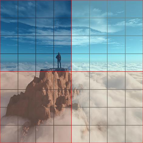
In actual shading scenes, there are often regions that are not adjacent in space but are related in color. The local window of image space and the local window of feature space have different concerns and different uses. figure 2 illustrates three methods for partitioning local self-attention windows: standard Window Self-Attention (WSA), Shifted Window Self-Attention (SWSA), and Feature Window Self-Attention (FWSA). These partitioning methods each have their own focus areas and overlapping aspects, contributing to the enlargement of receptive fields for individual patches.

Both Swin and BOAT models have the potential to improve model accuracy and generalization while reducing the computational cost of the Transformer. These models have shown excellent performance in image classification, object detection, and semantic segmentation applications. However, so far, there are no researchers applied it to interactive image colorization tasks.

(a) Windows Self-Attention (WSA)	(b) Shifted Windows Self-Attention (SWSA)	(c) Feature Windows Self-Attention (FWSA)
Figure 2. Three ways to divide local self-attention windows

2.3 Pixel brightness similarity

Levin et al. [1] were pioneers in the field of image colorization and introduced the concept that pixels with similar grayscale values should also have more similar colors. They established a weight function for pixel t and its neighboring pixel c as follows:

\( ω_{tc}∝e^{-\frac{(N(t)-N(c))^{2}}{2σ_{t}^{2}}} \) (3)

where, \( N(∙) \) represents the pixel neighborhood, \( σ_{t}^{2} \) is the brightness variance of the neighborhood pixels centered around pixel \( t \) , and the weight function satisfies the equation \( \sum_{c∈N(t)}^{} ω_{tc}=1 \) . If \( ω_{tc} \) is smaller, it indicates a greater color difference between pixels \( t \) and \( c \) ; otherwise, the colors of the two points are closer. Levin et al.'s method has been proven to produce excellent colorization results and laid the foundation for subsequent traditional image colorization methods [20-23]. They, along with other researchers, share a similar perspective and have introduced more complex mathematical tools to enhance colorization quality, such as variational methods and partial differential equations.

3 Proposed Method

3.1 Overall structure of the proposed method

Figure 3 illustrates the overall architecture of our model in this paper. We begin by preparing a grayscale image, denoted as \( I_{g}∈R^{H×W×1} \) and a color hint image , denoted as \( I_{hint}∈R^{H×W×3} \) The color hint image is created by adding several colored pixel blocks to the original image, following the standard size of 2×2 pixels as set by Zhang [7]. Next, their color spaces are converted from RGB to Lab, where L represents the luminance value, and a and b are the two chroma channels. Since the grayscale image contains only luminance information and lacks chroma information, its size remains \( I_{g}∈R^{H×W×1} \) . For the color hint image, the luminance information is retained from \( I_{g} \) at corresponding positions, while the chroma information is represented using the a and b channels. In the ab channels, all non-hinted regions are filled with zeros, resulting in the chroma information for the user's hint image, denoted as \( \widetilde{I}_{hint}∈R^{H×W×2} \) . The merging of these two images yields the image information \( X_{0}∈R^{H×W×3} \) in the Lab color space:

\( X_{0}=I_{g}⨁\widetilde{I}_{hint} \) (4)

where \( ⨁ \) is the channel-wise concatenation. Following this, the grayscale image with color hints is subjected to Patch Embedding, involving the following steps: the image gets divided into a series of patches, and each patch goes through feature extraction and mapping into a one-dimensional sequence, treated as a visual token. Initially, the patch size is set to 4×4, denoted as \( P_{1}=4 \) , resulting in each patch having a feature dimension of \( C=3×P_{1}^{2} \) , while the image information \( X_{1} \) has dimensions \( (\frac{H}{P_{1}},\frac{W}{P_{1}},3×P_{1}^{2}) \) . \( X_{1} \) is then employed as input and processed through our improved Hierarchical Transformer Encoder. In this encoder, as depicted in figure 3, the patch size changes at each stage, with a total of 4 stages. The final output feature information \( X_{4} \) has dimensions \( (\frac{H}{32},\frac{W}{32},3×32^{2}) \) , and at this stage, the patch size is \( P_{4}=32 \) .

The output image resolution, \( \widetilde{I}_{hint}∈R^{H×W×2} \) , is only 1/32 of the original image, so it is necessary to upsample the output feature image \( X_{4} \) to obtain a full-resolution color image [24]. The DUpsampling [25] technique, which is a more concise and efficient upsampling method, has been enhanced by the model. DUpsampling achieves upsampling by learning sub-pixel convolutions and can rearrange an image with dimensions \( (\frac{H}{P},\frac{W}{P},3×P^{2}) \) into the shape \( (H,W,3) \) to obtain a full-resolution image. To further mitigate the artifacts and color bleeding caused by DUpsampling, a convolutional layer with a receptive field of 3 is added as a local stabilizing layer between the Transformer and DUpsampling modules. This local stabilizing layer ensures smoother upsampling. Section 4.5 of this paper will include a set of ablation experiments to validate the effectiveness of the convolutional layer as a local stabilizing layer.

For the output result of upsampling, the a and b chrominance channels are retained, and channel fusion is carried out with the image \( I_{g} \) with the original brightness channel to obtain the final color prediction result \( I_{pred} \) :

\( I_{pred}=I_{g}⊕I_{ab} \) (5)

where \( ⨁ \) is the channel-wise concatenation. \( I_{g} \) represents the grayscale image information, and \( I_{ab} \) represents the calculated a and b chromaticity channel information.

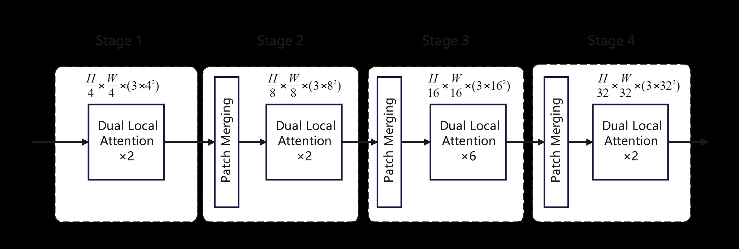Figure 3. Hierarchical Vision Transformer structure

3.2 Hierarchical Transformer

The hierarchical Transformer structure mentioned earlier, as shown in figure 3, operates with 4×4-sized patches. Tokens are input into the Dual Local Self-Attention Transformer module, which goes through both image space local self-attention and feature space local self-attention calculations sequentially. This process is referred to as "Stage 1."

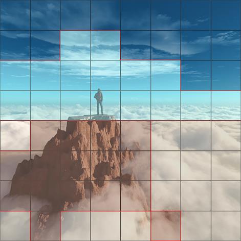
Next, the patch size is increased to 8×8 through a patch merging layer, reducing the length of the token sequence by 4 times and increasing the output channels by a corresponding factor of 4. It's worth noting that in the Swin model [13] design, at this point, there's an additional 1x1 convolution operation to reduce the channel dimension by half. However, in this model, this step is omitted to retain more channel information, which will be useful for later color resolution upsampling. This idea will be further validated in a set of ablation experiments in Section 4.5. The process of Patch Merging in the Swin model and our model is depicted in figure 4. Following this, tokens are applied to dual local self-attention Transformer blocks, referred to as "Stage 2". This process is repeated two more times until Stage 4, which outputs a resolution of \( (\frac{H}{32},\frac{W}{32}) \) with \( 3×32^{2} \) channels.

Figure 4. Patch Merging structure and subsequent size changes

3.3 Dual Local Self-Attention

In the standard Transformer architecture, global self-attention operations have quadratic computational complexity with the number of tokens, rendering them unsuitable for many high-resolution visual tasks with numerous tokens. To streamline computation and effectively capture inter-region relationships within an image, a Dual Local Self-Attention Transformer module is introduced in this paper, as shown in figure 5. It consists of three core components: the Windows Local Self-Attention (WSA) module, the Shifted Windows Self-Attention (SWSA) module and the Feature Windows Self-Attention (FWSA) module.

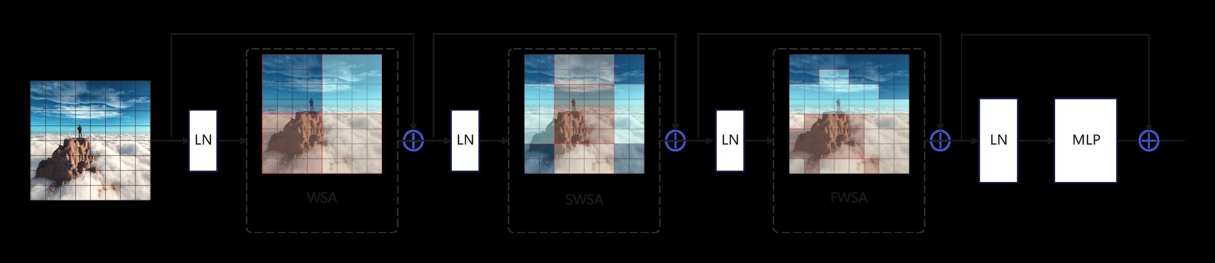Figure 5. Dual Local Self-Attention structure

The first step in performing local self-attention computation is to divide the image into non-overlapping local windows, and each token computes self-attention only within its window. However, if self-attention computation is restricted to non-overlapping regions, a token cannot establish connections with information outside its window. To facilitate cross-window connections, the shifted windows approach is adopted, where there is partial overlap between windows before and after shifting, and tokens are computed alternately following two different window partitioning rules. Although this approach significantly improves efficiency, it focuses only on connections between nearby regions. In the field of image colorization, similar colors may not necessarily be in spatial proximity.

To tackle this issue, the Feature Windows Self-Attention (FWSA) module is introduced in the paper. It operates based on feature similarity, where patches with high feature similarity are grouped into a local window. Self-attention computation is then performed within this new window. Consequently, a patch can establish connections with patches from the previous and subsequent windows, granting it access to a larger receptive field, akin to achieving global attention. The paper illustrates the two different window partitioning strategies in figure 2, each with its respective focus.

A complete Dual Local Self-Attention Transformer block is formed by adding Layer Normalization (LN) modules and Multi-Layer Perceptron (MLP) modules before and after the two local self-attention modules. The calculation for input token sequences through this Transformer encoder is as follows:

\( z_{l}^{ \prime }=WSA(LN(z_{l-1}))+z_{l-1} \) (6)

\( z_{l}^{ \prime \prime }=SWSA(LN(z_{l}^{ \prime }))+z_{l}^{ \prime } \) (7)

\( z_{l}^{ \prime \prime \prime }=FWSA(LN(z_{l}^{ \prime \prime }))+z_{l}^{ \prime \prime } \) (8)

\( z_{l+1}=MLP(LN(z_{l}^{ \prime \prime }))+z_{l}^{ \prime \prime \prime } \) (9)

Where \( LN(∙) \) indicates the layer normalization and \( MLP(∙) \) the multi-layer perceptron. \( WSA(∙) \) , \( SWSA(∙) \) and \( FWSA(∙) \) respectively represent the three local window self-attention modules shown in figure 5, and the output is \( z_{l}^{ \prime } \) , \( z_{l}^{ \prime \prime } \) and \( z_{l}^{ \prime \prime \prime } \) in layer \( l \) , \( z_{l+1} \) represents the input features of the next layer. Since self-attention does not utilize any position-related information, position encoding \( E_{pos} \) is added to the input of the attention layer and relative position biases [26]. Therefore, the calculation for the attention layer is as follows:

\( Attention(Q,K,V)=softmax(\frac{QK^{T}}{\sqrt[]{d}}+B)V \) (10)

where \( Q,K,V∈R^{N×d} \) are the query, key and value matrices . \( B∈R^{N×N} \) is the relative positional bias. \( N=HW/P^{2} \) is the number of input tokens, \( d=3×P^{2} \) is the hidden dimension.

Based on the existing ViT architecture [27], the MLP module consists of two fully connected layers. The first layer increases the feature dimension from \( C \) to \( rC \) , and the second layer reduces it back from \( rC \) to \( C \) . By default, \( r \) is set to 4.

3.4 Feature-space local attention

The feature-local attention mechanism classifies tokens based on the content of the tokens themselves. To enable efficient parallel processing on GPU platforms, this paper employs a multi-level binary clustering approach [17]. It performs \( K \) -level clustering, and at each level, a balanced binary clustering is performed, dividing a group of tokens into two equal sets. Suppose an image has \( N \) tokens. At the first level, these tokens are split into two subsets, each containing \( N∕2 \) tokens. At the \( k \) -th level, there will be \( 2k \) subsets, each containing \( N∕2k \) tokens.

Similar to K-means clustering, this method relies on cluster centers. In a set of tokens, two cluster centers, denoted as \( c_{1} \) and \( c_{2} \) , are established. The distance between each token \( t_{i} \) and the two cluster centers is compared, represented as \( r_{i} \) :

\( r_{i}=\frac{s(t_{i},c_{1})}{s(t_{i},c_{2})} \) (11)

where, \( s(t,c) \) represents the similarity between tokens. In the works of Roy and Yu [16, 17], cosine similarity is commonly used for calculating similarity, which is a widely accepted standard. However, for grayscale image colorization, this paper proposes a more fitting brightness similarity, \( s(t,c) \) , based on Levin et al.'s pixel neighborhood weight function [1]. In the experimental section in 4.5, we will compare the impact of choosing these two similarity measures to validate the effectiveness of the proposed brightness similarity in this paper. \( s(t,c) \) only requires a qualitative comparison of the distance between token \( t \) and the two cluster centers and does not require precise quantitative calculations. Therefore, the weight function \( ω_{tc} \) is simplified to:

\( s(t,c)=(N(t)-N(c))^{2} \) (12)

Where \( N(∙) \) represents the neighborhood of tokens. The smaller \( s(t,c) \) is, the more similar the information between token \( t \) and cluster center \( c \) . Otherwise, if \( s(t,c) \) is larger, the information difference between the token and the cluster center is greater. Each token \( t_{i} \) and its corresponding distance ratio \( r_{i} \) are sorted in ascending order. The tokens in the first half of the sorted list are assigned to cluster \( c_{1} \) , while those in the second half are assigned to cluster \( c_{2} \) . The process is repeated for the two sets of tokens until the number of tokens matches that in the corresponding SWSA module's local window. Finally, multi-head self-attention calculations are performed on the tokens within each set.

3.5 Objective Function

Our model is trained using the Huber loss [27] between the predicted image and the original color image in the CIELab color space. Our goal is to optimize the overall Huber loss. The loss function is defined as follows:

\( L_{Huber}=\begin{cases}\frac{1}{2}(I_{pred}-I_{ori})^{2} |I_{pred}-I_{ori}|≤δ|I_{pred}-I_{ori}|-\frac{1}{2}δ^{2} |I_{pred}-I_{ori}|>δ\end{cases} \) (13)

where \( L_{Huber} \) , \( I_{pred} \) and \( I_{ori} \) represent huber loss, the predicted image and the original color image. The hyperparameter \( δ \) plays a certain selection role in this formula. When \( δ~0 \) , Huber loss tends to MAE, and when \( δ~∞ \) , Huber loss tends to MSE, in this model we take \( δ=1 \) .

4 Experiments

4.1 Datasets

The experiments were conducted using the ImageNet 2021 dataset as the training set, which comprises over 1.2 million annotated images spanning 1000 categories. The model in this paper is trained in a self-supervised manner, and it does not utilize any classification labels during training. To assess the model's generalization capabilities, four different datasets from various domains were chosen for evaluation. These datasets are ImageNet ctest10k, Oxford 102flowers, CUB-200, NCD datasets [29], and no additional fine-tuning was applied to any of the validation datasets.

ImageNet ctest10k: This dataset is a subset of the ImageNet validation set, consisting of 10,000 color images. It doesn't contain any images from the ImageNet-1k dataset and is widely used as a standard validation set for evaluating grayscale image colorization models. It serves as the primary validation set for comparing results in this paper.

Oxford 102-flowers Dataset: This dataset provides 102 different categories of flowers, with each category containing around 40 to 258 images, totaling 8,189 images.

CUB-200 Dataset: The CUB-200 dataset includes 200 different categories of birds, with each category having around 40 to 60 images, resulting in approximately 12,000 images.

NCD Dataset: The NCD dataset encompasses over 6,000 images of various fruit categories, including lemons, strawberries, apples, bananas, oranges, and more.

These datasets were used to evaluate the performance of the model across different domains and scenarios.

4.2 evaluation indices

In this paper, the primary evaluation metric used is Peak Signal-to-Noise Ratio (PSNR) and Structure Similarity Index Measure (SSIM). PSNR is a common method for assessing the similarity between a reconstructed image and the original image, with higher values indicating smaller differences between the reconstructed and original images. In grayscale image colorization tasks, PSNR is used to measure the similarity between the colorized image and the original color image. It needs to be defined by Mean Squared Error (MSE). Let \( I(i,j) \) and \( K(i,j) \) represent the original image and the processed image respectively, and \( M×N \) represents the image size. MSE can be written as,

\( MSE=\frac{1}{mn}\sum_{i=o}^{m-1} \sum_{i=0}^{n-1} ‖I(i,j)-K(i,j)‖^{2} \) (14)

Then PSNR is defined as,

\( PSNR=10∙log_{10}{(\frac{MAX_{I}^{2}}{MSE})} \) (15)

where \( MAX_{I} \) is the maximum possible pixel value of the image. If each pixel is represented by an 8-bit binary, that would be 255.

SSIM is also a full-reference image quality evaluation index, which measures image similarity from three aspects: brightness, contrast, and structure. SSIM [30] is usually calculated as,

\( SSIM(x,y)=\frac{(2μ_{x}μ_{y}+C_{1})(2σ_{xy}+C_{2})}{(μ_{x}^{2}+μ_{y}^{2}+C_{1})(σ_{x}^{2}+σ_{y}^{2}+C_{2})} \) (16)

where \( x,y \) represent the original image and the processed image respectively, \( μ_{x}, μ_{y} \) respectively represent the average value of \( x,y \) , \( σ_{x}^{2}, σ_{y}^{2} \) respectively represent the variance of \( x,y \) , and \( σ_{xy} \) represents the covariance of \( x,y \) .

In addition to PSNR and SSIM, the paper also uses Patch Errors Variance (PEV) as an auxiliary evaluation metric in comparative experiments. PEV is calculated as the variance of the MSE for each image patch. Lower PEV values indicate smoother accuracy across different regions, resulting in better colorization quality with fewer artifacts such as visual noise and color bleeding. It's worth noting that PEV can only be calculated for models based on the ViT framework, while many interactive colorization algorithms are based on CNNs or Generative Adversarial Networks (GANs). Therefore, PEV comparisons are conducted in the paper's ablation experiment section. The higher the psnr and ssim values, the lower the pev value, and the better the image colorization quality.

4.3 Implementation Details

The experimental environment in this paper is based on a 64-bit Ubuntu 21.04 system with CUDA version 11.4, cuDNN version 8.4, Python version 3.8, an NVIDIA RTX-5000 GPU with 16GB of VRAM, and 128GB of system memory.

Regarding the specific parameters for designing the Transformer encoder, the paper follows the configurations of Swin-S and Swin-T [13], implementing two sets of models: Ours-S and Ours-T. The Ours-S model has more parameters, while the Ours-T model is a more lightweight version. During training, the images are initially resized to a resolution of 224×224, and the initial patch size is set to 4. The paper uses the AdamW optimizer [31] with a learning rate of 0.0005, managed by a cosine annealing scheduler [32]. For the colorization hints, 2×2 pixel blocks are used, and 10 random points are selected.

Training phase: We use the ImageNet 2021 dataset for training, the color images in the data set are grayscaled, and then we randomly select several coordinate points (usually 10, more and less quantities also tried, each dot size is 2×2 pixels) on each grayscale image and add the color prompt information of the original image. The model performs coloring based on these prompt information, and compares the coloring results with the original image to continuously learn iteratively.

Testing phase: The images in the test set are processed in the same way as in the training phase. Each comparison model is colored according to the same prompt information and finally compared with the original image.

4.4 Implementation Details

The paper compares the proposed model with five mainstream algorithms in the point-interactive colorization domain. These algorithms are Zhang et al.'s iDeepColor model [7], Yin et al.'s SWF model [9], Su et al.'s InstColor model [8], Yun et al.'s iColoriT model [11] and Lee et al.'s A-ColViT model [12]. It should be noted that the InstColor model of Su et al. [9] is originally an unconditional colorization model. Yun et al. extended it to the corresponding point interactive colorization model [11]. The InstColor model compared in this article is actually an extended version of Yun et al. We evaluate our network on multiple datasets, as shown in table 1. GFLOPs, PSNR, SSIM and the time cost of image colorization (measured in milliseconds) are used as our metrics. We were not able to measure the number of parameters for Yin et al. [9] since the method is not a learning-based model.

Table 1. Objective evaluation on different datasets

A higher PSNR value indicates better image quality. In this study, the Ours-S model consistently achieved thehighest PSNR values across all four datasets, while the Ours-T model exhibited slightly lower PSNR values compared to iColoriT. Compared to iColoriT-S, Ours-S shows a significant improvement in GFLOPs and time costs. The parameter count and time costs of the lightweight models A-ColViT and Ours-T are roughly equivalent. A-ColViT achieves a good balance between colorization performance and lightweight design. It's worth noting that the iColoriT model is built upon the ViT-B architecture [10], whereas our two models in this paper adhere to the configurations of Swin-S and Swin-T [13]. As a result, our models have smaller model parameter sizes and computational requirements, as detailed in table 2.

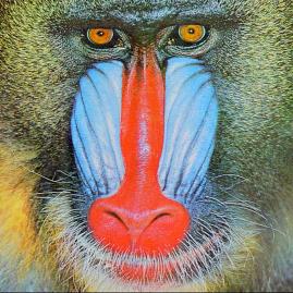
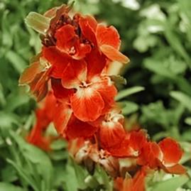
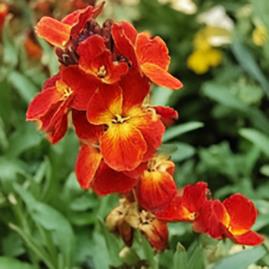
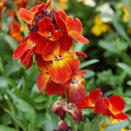
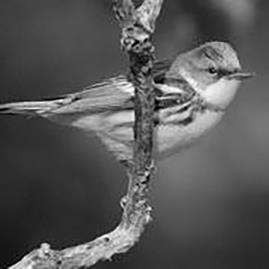
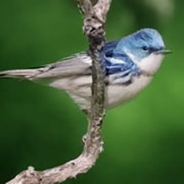
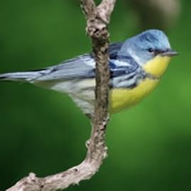
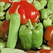
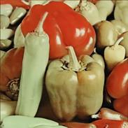
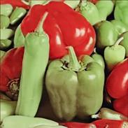
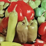
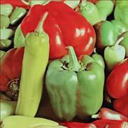
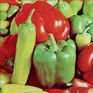
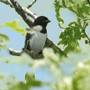
The comparative results of the colorization performance between our model, Zhang et al.'s iDeepColor model, and Yun et al.'s iColoriT model are illustrated in figure 6. Zhang first introduced deep learning-based methods for interactive image colorization in 2017, while iColoriT by Yun, proposed in 2022, currently represents the state-of-the-art in colorization performance. Subjectively, it is evident that both iDeepColor and iColoriT models exhibit varying degrees of color bleeding artifacts, whereas our model excels in preserving color edge details, resulting in a more visually realistic output.

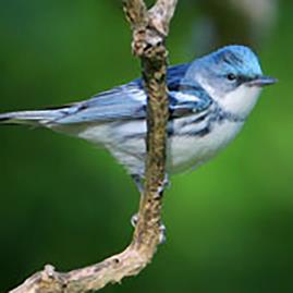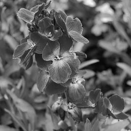
(a) Input	(b)iDeepColor	(c)iColoriT	(d) Ours-S	(e) Truth
Figure 6. Colorization comparison effect with different models

Table 2. Comparison of the complexity of various ViT

4.5 Ablation Study

In this section, based on the Ours-S model as the baseline, we conducted five sets of ablation experiments to investigate the impact of three aspects: the choice of the local stabilizing layer, whether the patch merging layer performs channel-wise convolution, and the selection of the feature space clustering metric.

Local Stabilizing Layer: The local stabilizing layer is placed between the Hierarchical Transformer Encoder and the DUpsampling modules. Its purpose is to mitigate artifacts caused by upsampling. Our model employs a convolutional layer with a receptive field of 3 as the local stabilizing layer. There are three contrast models: Model 1: No local stabilizing layer. Model 2: A simpler linear layer as the local stabilizing layer. Model 3: A more complex local self-attention layer as the local stabilizing layer.

Patch Merging Layer: In the patch merging layer of the Hierarchical Transformer module, Swin models include an additional 1x1 convolution in the channel dimension. This is done to align with widely used CNN architectures and enhance model compatibility. On the other hand, the Ours-S model preserves more channel information to improve upsampling. There is one comparative model: Model 4: Similar to Swin models, retains the convolution operation on the channel dimension and adjusts the upsampling rate accordingly in the DUpsampling stage.

Feature Space Clustering Metric: In feature-based local space clustering, where patches are organized for local self-attention calculations, the Ours-S model utilizes the suggested luminance similarity metric. There is one comparative model: Model 5: Utilizes the more common cosine similarity as the clustering metric. These ablation experiments were conducted using the ImageNet ctest10k as the validation set, and the results are shown in table 3.

Table 3. Results of ablation experiments

Where B-PSNR stands for Boundary Peak Signal-to-Noise Ratio, akin to PEV, which can only be computed in models based on the ViT framework. A higher PSNR implies a smaller difference between the reconstructed image and the original image, while a lower PEV signifies smoother precision in generated images, with fewer artifacts such as pseudo-contours and color bleeding. Referring to table 3, we can infer the colorization quality of the control models in the following order: Model 3 > Model 2 > Model 4 > Model 5 > Model 1. For ease of visual comparison, the colorization results are presented in figure 7 accordingly. Combining the subjective impressions from figure 7 with the objective indicators in table 3, it's evident that the image quality reflected by the objective metrics is largely consistent. Model 1, without a local stabilizing layer, exhibits a notable decrease of 2.07 dB in PSNR and a 4.94 increase in PEV, significantly impacting image quality.

Using a convolutional layer as the local stabilizing layer, as in Model 2, and employing a local attention layer as in Model 3, yields slight improvements compared to the linear layer. This design is straightforward and effective. In Model 4, following the original Swin model by applying an additional channel-wise convolution after each hierarchical stage, there's a slight decline in image quality. Model 5, utilizing the simpler cosine similarity as a feature space clustering metric, experiences a significant drop in image colorization quality, only surpassing Model 1 without a local stabilizing layer. This underscores the effectiveness of the proposed brightness similarity metric.

(a) Model 1	(b) Model 5	(c) Model 4	(d) Model 2	(e) Model 3	(f) Ours-S	(g)Truth
Figure 7. Comparison of model colorization effects in ablation experiments

5 Conclusion

This paper improves the ViT framework for the task of point-wise interactive grayscale image colorization. To address the computational inefficiency of Transformers in the colorization domain, the global self-attention mechanism is replaced with a dual local self-attention mechanism. This is achieved by establishing spatial relationships between patches through sliding local windows and creating feature connections through clustering similar patches. Furthermore, the paper introduces brightness similarity as a targeted replacement for the more common cosine similarity, tailoring it for image colorization. DUpsampling techniques are applied during the upsampling phase of Transformer output, and a local stabilizing layer is added to alleviate artifacts and color bleeding associated with upsampling. In comparison to colorization methods based on standard Transformer models, this approach not only reduces parameter count by 40% and computational complexity by 80% but also exhibits superior colorization performance across multiple datasets compared to mainstream algorithms.

While our proposed algorithm demonstrates several advantages in the context of interactive image colorization, it does have limitations, particularly when colorizing small objects. Achieving satisfactory colorization in small object regions often requires a substantial amount of meticulous user-provided colors. This challenge becomes more prominent when dealing with grayscale information that is highly similar. Given that the model operates without leveraging any semantic labels and is trained in a self-supervised manner, a viable avenue for improvement is to explore direct training using segmentation labels for point-interactive colorization models. An alternative approach involves granting users complete creative freedom, where the model's role is limited to identifying potential regions of dissimilar colors, serving as prompts for the user. In summary, we believe that the algorithm can effectively assist users in images colorization.

References

[1]. Levin A, Lischinski D, Weiss Y. Colorization using optimization[M]. ACM SIGGRAPH 2004 Papers. 2004: 689-694.
[2]. Welsh T, Ashikhmin M, Mueller K. Transferring color to greyscale images[C]//Proceedings of the 29th annual conference on Computer graphics and interactive techniques. 2002: 277-280.
[3]. Hu H, Li F. Image colourisation by non‐local total variation method in the CB and YIQ colour spaces[J]. IET Image Processing, 2018, 12(5): 620-628.
[4]. Deshpande A, Rock J, Forsyth D. Learning large-scale automatic image colorization[C]//Proceedings of the IEEE international conference on computer vision. 2015: 567-575.
[5]. Iizuka S, Simo-Serra E, Ishikawa H. Let there be color! Joint end-to-end learning of global and local image priors for automatic image colorization with simultaneous classification[J]. ACM Transactions on Graphics (ToG), 2016, 35(4): 1-11.
[6]. Qin X, Li M, Liu Y, et al. An efficient coding‐based grayscale image automatic colorization method combined with attention mechanism[J]. IET Image Processing, 2022, 16(7): 1765-1777.
[7]. Zhang R, Zhu J Y, Isola P, et al. Real-time user-guided image colorization with learned deep priors[J]. arXiv preprint arXiv:1705.02999, 2017.
[8]. Yin H, Gong Y, Qiu G. Side window filtering[C]//Proceedings of the IEEE/CVF Conference on Computer Vision and Pattern Recognition. 2019: 8758-8766.
[9]. Su J W, Chu H K, Huang J B. Instance-aware image colorization[C]//Proceedings of the IEEE/CVF Conference on Computer Vision and Pattern Recognition. 2020: 7968-7977.
[10]. Dosovitskiy A, Beyer L, Kolesnikov A, et al. An image is worth 16x16 words: Transformers for image recognition at scale[J]. arXiv preprint arXiv:2010.11929, 2020.
[11]. Yun J, Lee S, Park M, et al. iColoriT: Towards Propagating Local Hints to the Right Region in Interactive Colorization by Leveraging Vision Transformer[C] //Proceedings of the IEEE/CVF Winter Conference on Applications of Computer Vision. 2023: 1787-1796.
[12]. Lee G, Shin S, Ko D, et al. A-ColViT: Real-time Interactive Colorization by Adaptive Vision Transformer[J]. 2023.
[13]. Vaswani A, Shazeer N, Parmar N, et al. Attention is all you need[J]. Advances in neural information processing systems, 2017, 30.
[14]. Liu Z, Lin Y, Cao Y, et al. Swin transformer: Hierarchical vision transformer using shifted windows[C]. Proceedings of the IEEE/CVF international conference on computer vision. 2021: 10012-10022.
[15]. Kitaev N, Kaiser Ł, Levskaya A. Reformer: The efficient transformer[J]. arXiv preprint arXiv:2001.04451, 2020.
[16]. Tay Y, Bahri D, Yang L, et al. Sparse sinkhorn attention[C]//International Conference on Machine Learning. PMLR, 2020: 9438-9447.
[17]. Roy A, Saffar M, Vaswani A, et al. Efficient content-based sparse attention with routing transformers[J]. Transactions of the Association for Computational Linguistics, 2021, 9: 53-68.
[18]. Yu T, Zhao G, Li P, et al. BOAT: Bilateral local attention vision Transformer[J]. arXiv preprint arXiv:2201.13027, 2022.
[19]. Gain M, Debnath R. A novel unbiased deep learning approach (dl-net) in feature space for converting gray to color image[J]. IEEE Access, 2023.
[20]. Yatziv L, Sapiro G. Fast image and video colorization using chrominance blending[J]. IEEE Transactions on image processing, 2006, 15(5): 1120-1129.
[21]. Chen Y, Zong G, Cao G, et al. Image colourisation using linear neighbourhood propagation and weighted smoothing[J]. IET Image Processing, 2017, 11(5): 285-291.
[22]. Kang S H, March R. Variational models for image colorization via chromaticity and crightness decomposition[J]. IEEE Transactions on Image Processing, 2007, 16(9): 2251-2261.
[23]. Jin Z M, Zhou C, Ng M K. A coupled total variation model withcurvature driven for image colorization[J], Inverse Problems and Imaging, 2016, 10(4): 1037-1055.
[24]. Shi W, Caballero J, Huszár F, et al. Real-time single image and video super-resolution using an efficient sub-pixel convolutional neural network[C]//Proceedings of the IEEE conference on computer vision and pattern recognition. 2016: 1874-1883.
[25]. Tian Z, He T, Shen C, et al. Decoders matter for semantic segmentation: Data-dependent decoding enables flexible feature aggregation[C]//Proceedings of the IEEE/CVF Conference on Computer Vision and Pattern Recognition. 2019: 3126-3135.
[26]. Hu H, Gu J, Zhang Z, et al. Relation networks for object detection[C]//Proceedings of the IEEE conference on computer vision and pattern recognition. 2018: 3588-3597.
[27]. Touvron H, Cord M, Douze M, et al. Training data-efficient image Transformers & distillation through attention[C]//International conference on machine learning. PMLR, 2021: 10347-10357.
[28]. Peter J Huber. Robust estimation of a location parameter. In Breakthroughs in statistics, pages 492–518. Springer, 1992.
[29]. Anwar S, Tahir M, Li C, et al. Image colorization: A survey and dataset[J]. arXiv preprint arXiv:2008.10774, 2020.
[30]. Wang Z, Bovik A C, Sheikh H R, et al. Image quality assessment: from error visibility to structural similarity[J]. IEEE transactions on image processing, 2004, 13(4): 600-612.
[31]. Ilya Loshchilov and Frank Hutter. Decoupled weight decay regularization. In International Conference on Learning Representations, 2018.
[32]. Loshchilov I, Hutter F. Decoupled weight decay regularization[J]. arXiv preprint arXiv:1711.05101, 2017.
Cite this article
Li,Y.;Bao,X.;Qiang,Z. (2024). Interactive image colorization method via dual local self-attention. Applied and Computational Engineering,68,258-272.
Data availability
The datasets used and/or analyzed during the current study will be available from the authors upon reasonable request.
Disclaimer/Publisher's Note
The statements, opinions and data contained in all publications are solely those of the individual author(s) and contributor(s) and not of EWA Publishing and/or the editor(s). EWA Publishing and/or the editor(s) disclaim responsibility for any injury to people or property resulting from any ideas, methods, instructions or products referred to in the content.
About volume
Volume title: Proceedings of the 6th International Conference on Computing and Data Science
© 2024 by the author(s). Licensee EWA Publishing, Oxford, UK. This article is an open access article distributed under the terms and
conditions of the Creative Commons Attribution (CC BY) license. Authors who
publish this series agree to the following terms:
1. Authors retain copyright and grant the series right of first publication with the work simultaneously licensed under a Creative Commons
Attribution License that allows others to share the work with an acknowledgment of the work's authorship and initial publication in this
series.
2. Authors are able to enter into separate, additional contractual arrangements for the non-exclusive distribution of the series's published
version of the work (e.g., post it to an institutional repository or publish it in a book), with an acknowledgment of its initial
publication in this series.
3. Authors are permitted and encouraged to post their work online (e.g., in institutional repositories or on their website) prior to and
during the submission process, as it can lead to productive exchanges, as well as earlier and greater citation of published work (See
Open access policy for details).