1. Introduction

Mobile robots, while working under real life conditions, must be capable of navigating and locating themselves in large, unknown environments. To do so, these robots are required to map their current environments to localize themselves in it, which is known as the SLAM (Simultaneous Localization and Mapping) problem [1]. A typical SLAM system consists of two modules: odometry and mapping, which are used to approximate the robot's current location and map its current environment. However, in such system, localization inevitably drift with time due to the sensor error accumulation [2]. Loop closure detection, a process which the robot detects and recognizes its returning to previously visited locations, plays a vital role in the fields of SLAM and robotic application. It helps eliminate the accumulated drift due to sensor errors, increasing the accuracy of localization and ensures more reliable navigation in autonomous driving [3]. Further, it can potentially enhance the process of re-localization within pre-build high-resolution map, facilitating immediate recovery from tracking failures and seamless reconstruction of the high-resolution map. This enhanced map can subsequently be utilized in diverse applications such as virtual reality (VR), augmented reality (AR), and motion/mission planning in autonomous driving [4]. In multi-robot collaboration, loop closure detection may contribute to aligning and associating sensory data from concurrent environment and merging two pre-build maps from two individual robots [5].

Loop closure detection methods for mobile robots can be primarily divided into visual-based and point cloud-based methods. Visual method is more frequently used in SLAM context for its low cost and widespread availability. By comparing visual features and semantic information between two visual images, it is able to determine whether an active loop closure has occur [6]. However, mere visual-based method cannot obtain the geometric and structural information of the environment, and is sensitive to environmental changes: lighting conditions, shadows, and seasonal changes can all alter the results of visual-based loop closure detection [7][8][9]. Hence, in search of a more stable and robust method for loop closure detection, there is a prevailing preference to utilize the point cloud data, often acquired by LiDAR [10]. Such method primarily focuses on developing and matching descriptors from geometric and structural information in current environment [9]. Nevertheless, there are still three inherent issues that existing point cloud-based method need to overcome. First, it must require a high resolution LiDAR scanner to operate, which is a currently high-cost sensor. Second, as shown in Figure 1, the point density in each LiDAR scan decreases along with increasing distance, meaning the density of a typical point cloud varies with distance, hence the descriptors might have varying accuracy. Finally, the numerous point data in a typical point cloud largely expands the cost of time for processing and computing point cloud information [3]. Hence, in order to achieve real-time and seamless loop closure, the point cloud-based method must implement an efficient and less time-consuming algorithm to transform point cloud data into distinctive descriptors.

To solve these technical challenges, in this study, we design a robust Bird's Eye View (BEV) descriptor that is invariant with point cloud densities, scanning pattern, and noise variance between different kind of LiDAR scanners. To achieve real-time and seamless loop closure detection, we further introduce an efficient algorithm that transforms point cloud data into such descriptors and retrieves possible candidates for loop closure through these descriptors. In conclusion, the main contribution of this work can be summarized as below:

• We integrate a robust BEV descriptor into a LiDAR-inertial-based odometer and form a complete SLAM system, suitable for long-term localization and mapping. The implementation is lightweight through a single C++ and is readily integrable to any existing SLAM framework.

• We evaluate our algorithm under multiple scenarios, both indoor and outdoor. Sufficient experimental results verify the effectiveness of our method.

• We extensively evaluate our method on both public and private datasets, and on different types of LiDAR scanner to demonstrate the adaptability of our proposed descriptor. The performance of our method is compared to a state-of-art descriptor, Scan Context [8], and exhibits a considerable improvement.

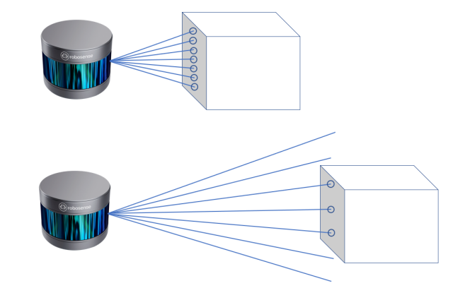
Figure 1. Point density varies from distance

2. Relative Work

Loop closure detection methods, as mentioned previously, are categorized into visual-based and LiDAR-based methods.

2.1. Visual-based Methods

Visual methods are more commonly used for loop closure detection in SLAM frameworks [8] [11] [12] [13]. However, unlike LiDAR-based methods, visual based loop closure detection are usually less robust against perceptual changes. FAB-MAP [8] proposed by Cummins et al. approaches to the problem by proposing a probabilistic generative model of place appearance. Although it does successfully account for perceptual aliasing in surrounding--low probability of revisiting due to indistinctive appearance, visual representation is still vulnerable to weather/lightness changes [14], limiting its real life performance. In contrast, our point cloud representation remains invariant under environment changes. Hence, the descriptor that we proposed is adaptive to different environment. SeqSLAM [15] from Milford et al. achieves loop closure detection with a far improved performance from FAB-MAP through sequential place recognition. Rather than determining a sole optimal match for a given image, SeqSLAM examines the best match location within every local navigation sequence, which proves to be resilient against environment changes. SRAL [16] fuses different features such as colors and lightness from an environment to represent its long-term appearance and transforms loop closure detection into a single regularized optimization problem.

2.2. LiDAR-based Methods

Since LiDAR sensor only extracts geometric information from its surrounding, most LiDAR-based methods exhibit strong resilience against environment and perceptual changes. LiDAR-based methods rely on key-point descriptors, in which nearby points of selected key-points are separated into different cells, and surrounding cells are then encoded into a histogram based on a shared pattern. However, most of these key-point descriptors are originally devised for 3D model part matching [8] and hence revealed limitations when used in loop closure detection context. The conditions of a point cloud deviate much from those of a 3D model. For instance, the density of a 3D model remains constant throughout the model, yet that of a point cloud varies through distance. Moreover, since derived from a real life environment, a point cloud contains more noises than a model. Both suggests that key-point descriptors are not suitable to use for loop closure detection. Scan Context [8] by Kim et al. is a non-histogram based descriptor from LiDAR scans. It transforms the 3D point cloud from various LiDAR scans into 2D visual representations through partitioning the ground areas into different bin based on point cloud top view azimuthal and radial direction. Then, these visual representations are being compared to determine whether loop closure has occur. However, such method stands on the strong assumption that the vehicle has no notable changes in the z-axis, which makes the descriptor sensitive to changes in roll and pitch angles. Our method is adaptive projection, which can be use in multiple extreme conditions such as in crowded urban areas, on a handheld device, in aerial mapping with large motions. SegMatch [17] developed a loop closure detection through deep learning and object segmentation. The training process of the network requires large datasets and hardware support (GPU acceleration). The method that we proposed requires only a workable CPU with no other specific needs for hardware to operate.

In this paper, we propose a robust and adaptive LiDAR-based descriptor that transforms a point cloud into a BEV image, which is then used to search for possible candidates of loop closure. Our method can be applied to variant SLAM contexts, unaffected by changes in environments or types of LiDAR sensors. The process of BEV image generation is inspired by Scan Context [8], which also increases the descriptor's resilience against azimuthal changes. In detail, our proposed method consists of three major component: BEV image generation that preserves the geometric and structural information of point cloud key-frames, retrieval that searches and verifies for possible loop closure candidates, and pose graph optimization according to the loop closure detection results.

3. Method

In this section, we describe how to construct an adaptive BEV descriptor from a 3D point cloud. First, we introduce the LiDAR odometry to extract point cloud key-frames. Next, we apply plane projection and space partition on the key-frames to generate our BEV descriptor. Finally, descriptor-based candidate retrieval and geometric verification are proposed for a complete loop closure detection pipeline. The overall pipeline of our method is depicted in Figure 2.

3.1. LiDAR-Inertial Odometry

Since our proposed method performs loop closure detection on point cloud key-frames, a LiDAR odometer is required to register point cloud from each LiDAR scans to the current key-frame. Then, a new key-frame is generated when a certain number of sub-frames accumulates. By combining data from different sensors, we can get a clearer picture of environment and thus output key-frames with a higher accuracy. Among the various methods available, we've picked the Extended Kalman Filter (EKF) to merge information from LiDAR and IMU sensors. Using EKF helps us map the environment more accurately and deal with difficult situations better. This is mainly because the EKF can handle complex calculations by simplifying them step by step, especially when we assume the errors are normally distributed.

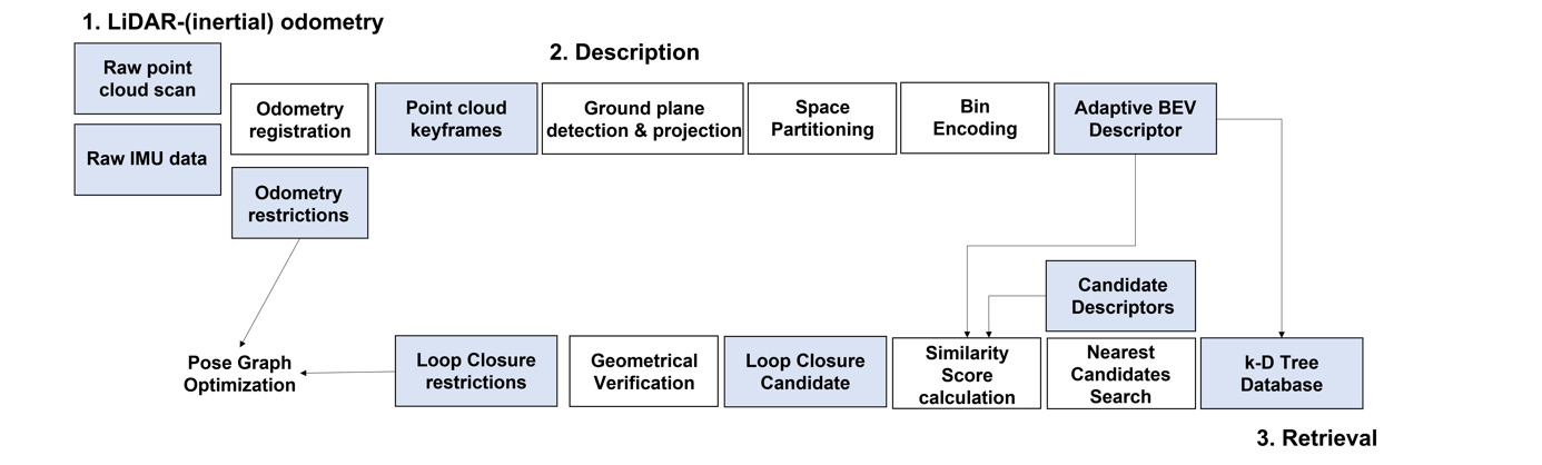
Figure 2. Method Overview. First, LiDAR scans are registered through an odometer based on extended kalman filter, and accumulates to form key-frames. Then, the ground plane is detect to project the points from the key-frame. Key-frames after plane projection will be partitioned and encoded to generate BEV descriptors. Candidates of loop closure are retrieved by their descriptor, then the final candidate is validated through ICP-based geometric verification. Once loop closure is triggered, its provided restrictions will be used for pose graph optimization.

3.1.1. State Definition. The state vector, x, is formulated as:

\( x=[\begin{matrix}{p^{T}} & {R^{T}} & {v^{T}} & b_{a}^{T} & b_{g}^{T} \\ \end{matrix}] \) (1)

Where:

p represents the position of the LiDAR in a global reference frame. This is the 3D location given by:

\( p=[x,y,z] \) (2)

Here, x, y, and z denote the coordinates in the east, north, and up directions, respectively.

R describes the orientation of the LiDAR in the global frame, represented as a rotation matrix:

\( R=[\begin{matrix}{r_{11}} & {r_{12}} & {r_{13}} \\ {r_{21}} & {r_{22}} & {r_{23}} \\ {r_{31}} & {r_{32}} & {r_{33}} \\ \end{matrix}] \) (3)

Each element \( {r_{ij}} \) of the matrix represents the cosine of the angle between the respective axes of the LiDAR’s local frame and the global frame.

v indicates the linear velocity of the LiDAR in the global frame:

\( v=[{v_{x}},{v_{y}},{v_{z}}] \) (4)

This showcases how fast the vehicle is moving and in which direction.

\( {b_{a}} \) stands for the accelerometer bias, which can drift over time and impact the accuracy of acceleration measurements:

\( {b_{a}}=[{b_{{a_{x}}}},{b_{{a_{y}}}},{b_{{a_{z}}}}] \) (5)

\( {b_{g}} \) represents the gyroscope bias, accounting for drifts that affect angular velocity measurements:

\( {b_{g}}=[{b_{{g_{x}}}},{b_{{g_{y}}}},{b_{{g_{z}}}}] \) (6)

3.1.2. Process Model. Building upon the state vector x defined earlier, which includes the position p, orientation R, velocity v, accelerometer bias \( {b_{a}} \) , and gyroscope bias \( {b_{g}} \) , the process model predicts the next state based on the current state and control inputs.

For LiDAR-Inertial odometry using EKF, the primary control inputs are the IMU measurements. These measurements, particularly angular velocities from the gyroscope and linear accelerations from the accelerometer, can be influenced by the biases \( {b_{a}} \) and \( {b_{g}} \) , respectively.

Given state vector x at time t, the state’s evolution to time \( t+Δt \) is predicted using the IMU readings. The accelerations a (adjusted for \( {b_{a}} \) ) and angular velocities \( ω \) (adjusted for \( {b_{g}} \) ), usually provided by the accelerometer and gyroscope, are integrated to estimate changes in position, velocity, and orientation.

\( \begin{matrix} & {p_{t+Δt}} {= p_{t}}+{v_{t}}Δt+\frac{1}{2}{a_{t}}Δ{t^{2}} & & \\ & {V_{t+Δt}}={v_{t}}+{a_{t}}Δt & & \\ & {R_{t+Δt}}={R_{t}}ΔR({ω_{t}}Δt) & & \\ & {b_{t+Δt}}={b_{t}} & & \\ \end{matrix} \) (7)

Here: p represents the position. v denotes the velocity. R is the rotation. b represents the two biases. a is the acceleration from the IMU. \( ω \) is the angular velocity from the gyroscope. \( ΔR \) (·)is a function that provides the rotation matrix increment given an angular velocity. Small angle approximations or Rodrigues’ formula [18] can be used to obtain this incremental rotation. The predicted state is denoted as .

3.1.3. Measurement Model. Upon obtaining the predicted state, , from the process model, we utilize the LiDAR scan data in conjunction with the previously constructed point cloud map to establish a measurement model to obtain updated state \( {\bar{x}_{t}} \) . The initial value of \( {\bar{x}_{t}} \) is the predicted state.

For a given LiDAR point, \( { ^{B}}{P_{i}} \) , in the LiDAR’s body frame, we first transform this point to the global frame:

\( { ^{G}}{P_{i}}={ ^{G}}{\bar{R}_{t}}{ ^{B}}{P_{i}}+{ ^{G}}{\bar{p}_{t}} \) (8)

Subsequently, the nearest plane with plane normal vector \( u_{i}^{ } \) and centroid \( { ^{G}}{q_{i}} \) corresponding to this point is identified, and a point-to-plane residual is constructed:

\( \begin{matrix}{z_{i}} =h({\bar{x}_{t}},{ ^{B}}{P_{i}}) & \\ =u_{i}^{T}{(^{G}}{P_{i}}-{ ^{G}}{q_{i}}) & \\ =u_{i}^{T}{(^{G}}{\bar{R}_{t}}{ ^{B}}{P_{i}}+{ ^{G}}{\bar{p}_{t}}-{ ^{G}}{q_{i}}) & \\ \end{matrix} \) (9)

To continue, the Jacobian \( {H_{t}} \) is computed by differentiating the state variables and is then evaluated at the current estimate of the state:

\( {H_{t}}=[-u_{i}^{TG}{\hat{R}_{t}}{⌊^{L}}{p_{i}}{⌋_{∧}},u_{i}^{T},{0_{1×3}},{0_{1×3}},{0_{1×3}}] \) (10)

Considering all n LiDAR measurement points collectively, the residuals \( {z_{i}} \) and the Jacobian matrix \( {H_{t}} \) are amalgamated as:

\( {z_{t}}=h({\bar{x}_{t}},{ ^{B}}P) =[ \begin{array}{c} h({\bar{x}_{t}},{ ^{B}}P{ _{1}}) \\ h({\bar{x}_{t}},{ ^{B}}P{ _{2}}) \\ ⋯ \\ h({\bar{x}_{t}},{ ^{B}}P{ _{n}}) \end{array} ] \)

(11)

\( {H_{t}}=[\begin{matrix}-u_{1}^{TG}{\bar{R}_{t}}{⌊^{L}}{p_{1}}{⌋_{∧}}, & u_{1}^{T}, & {0_{1×3}}, & {0_{1×3}}, & {0_{1×3}} \\ -u_{2}^{T}G{\bar{R}_{t}}{⌊^{L}}{p_{2}}{⌋_{∧}}, & u_{2}^{T}, & {0_{1×3}}, & {0_{1×3}}, & {0_{1×3}} \\ & ... & & & \\ -u_{n}^{TG}{\bar{R}_{t}}{⌊^{L}}{p_{n}}{⌋_{∧}}, & u_{n}^{T}, & {0_{1×3}}, & {0_{1×3}}, & {0_{1×3}} \\ \end{matrix}] \)

Lastly, the pose is optimized to minimize these residuals. As a result, we obtain the updated state \( {\bar{x}_{t}} \) of the LiDAR observation model.

3.1.4. State Update. After deducing the prior pose estimate \( {\hat{x}_{t}} \) and the associated covariance \( {\hat{p}_{t}} \) under the constant velocity model assumption, we incorporate n valid measurements from the latest LiDAR frame. Utilizing this data, we form a Maximum A Posteriori (MAP) estimation to enhance the precision of our current state estimate. The optimization problem can be formulated as:

\( _{ {x_{t}}}^{min}(∥{x_{t}}⊟ {\hat{x}_{t}}∥_{{\hat{P}_{t}}}^{2}+\sum _{i=1}^{n} ∥{z_{i}}-{H_{i}}\cdot ({x_{t}}⊟{\bar{x}_{t}})∥_{{w_{i}}}^{2}) \) (12)

Given \( n \) valid LiDAR measurements, we consolidate them as \( {H_{t}}={[H_{1}^{T},H_{2}^{T},...,H_{n}^{T}]^{T}} \) and \( {W_{t}}=diag({{{w_{1}}{,w_{2}}{, ...,w_{n}}_{ }}_{ }}) \) . The Kalman gain, \( {K_{t}} \) , which represents the weight of the measurement relative to the state prediction, is then computed as:

\( {K_{t}}={\hat{P}_{t}}H_{t}^{T}({H_{t}}{\hat{P}_{t}}H_{t}^{T}+{W_{t}}{)^{-1}} \) (13)

Lastly, the Kalman gain \( {K_{t}} \) is employed to procure the optimal updated state \( {x_{t}} \) and its associated covariance matrix \( {P_{t}} \) :

\( {x_{t}}={\hat{x}_{t}}⊞{K_{t}}({z_{t}}-h({\hat{x}_{t}},{ ^{B}}P)) \) (14)

\( {P_{t}}=(I-{K_{t}}{H_{t}}){\hat{P}_{t}} \)

The updated state \( {x_{t}} \) offers a more accurate representation of the system’s current state by combining prior knowledge and current measurements, thus refining the overall pose estimation.

3.2. BEV Descriptor

3.2.1. Ground Plane detection. To achieve an adaptive and robust descriptor to changes in roll and pitch angle, we first perform ground plane detection for each key-frame of the entire 3D point cloud. First, we divide the key-frame point cloud into various voxels of certain sizes (e.g., 1m). For each voxel, we want to find a best fitting plane \( π \) with crosspoint c and a normal vector n for the group of points \( {x_{i}} \) \( (i=1,…,N) \) . Therefore, the problem is to mathematically solve:

\( _{c,n,∣∣n∣∣=1}^{ min}\sum _{i=1}^{N} (({x_{i}}-c{)^{T}}n{)^{2}} \) (15)

Notice that is the value of \( n \) will not affect the domain of \( n \) , hence solving \( c \) is equivalent to finding a point that minimizes the sum of squares of the distances from other points to it, which happens to be the definition of the centroid. Then, to solve \( n \) , let \( {y_{i}}={x_{i}}-c \) , the expressions becomes:

\( _{n,∣∣n∣∣=1}^{ min}\sum _{i=1}^{N} (y_{i}^{T}n{)^{2}}= _{n,∣∣n∣∣=1}^{ min}{n^{T}}(Y{Y^{T}})n \) (16)

Where Y is a \( 3×N \) matrix from the concatenation of vector \( y_{i}^{ } \) . By the definition of scatter matrix, Y \( {Y^{T}} \) here is the scatter matrix of points \( x_{i}^{ } \) . Denote Y \( {Y^{T}} \) as S and with constraint \( {n^{T}}n \) =1, apply Lagrange multiplyer to find the local minimum of the Lagrange function:

\( L(n,λ)≡f(n)-λ({n^{T}}n-1) \) (17)

Finally, when the eigenvector and eigenvalues of the matrix S are assigned to n and \( λ \) respectively, the function is able to satisfy:

\( Sn=λn \) (18)

Where \( f(n) \) is able to reach its local extremum.

From the foregoing processes, we calculate the point scatter matrix S for each voxel:

\( \bar{x}=\frac{1}{N}\sum _{i=1}^{N} {x_{i}} \) ; \( S=\sum _{i=1}^{N} ({x_{i}}-\bar{x})({x_{i}}-\bar{x}{)^{T}} \) (19)

Apply eigendecomposition to matrix S, and let \( {λ_{k}} \) denote the \( K \) -th largest eigenvalue. According to the plane criterion principle proposed by STD [9]:

\( {λ_{3}} \lt {σ_{1}} and{ λ_{2}} \gt {σ_{2}} \) (20)

where \( {σ_{1}} \) and \( {σ_{2}} \) are pre-set hyperparameters. Using this criterion, we can determine if the points within a voxel can form a plane. Subsequently, we initialize a plane by selecting any such voxel and search for its neighboring voxels. If the neighboring voxels are on the same plane (has the same plane normal direction within a threshold distance), they are included into the expanding plane.

3.2.2. BEV Image Generation. Our BEV Image Generation method is inspired by Scan Context [8], which azimuthally and radially partitions the point cloud and transforms geometric shape of the point cloud around a local key point into an pixel image. Since Scan Context assumes that all LiDAR points lay on a plane perpendicular to the z-axis, its proposed descriptor is less resilient against disturbance in row and pitch angles. Our method effectively addresses this problem by selecting the best-fit plane as a reference. Given a frame of point cloud \( P=\lbrace {p_{1}},{p_{2}},...,{p_{N}}\rbrace \) and its best-fit plane \( π \) with crosspoint c and a normal vector n, we first projects the various points in the point cloud onto the ground plane by calculating the Euclidean distance d between the point and the plane:

\( D({p_{i}})={n^{T}}({p_{i}}-c), where i=1,2,...,N \) (21)

To project the points onto the plane, we rotate the point cloud frame until the z-axis of its local coordinate coincides with the normal vector of the plane. After such transformation, the z-coordinate of every point within the frame will become the calculated point-to-plane distance. Using the key point \( c=(\overline{x},\overline{y}) \) , each projected point \( {(x_{i }} \) , \( {y_{i }} \) )is transformed into polar coordinates \( ({r_{i}},{θ_{i}}) \) with respect to the key point and the plane by:

\( {r_{i}}=\sqrt[]{({x_{i}}-\overline{x}{)^{2}}+({y_{i}}-\overline{y}{)^{2}}},{θ_{i}}=atan2({y_{i}}-\overline{y},{x_{i}}-\overline{x}) \) (22)

After projection, our goal is to partition the scan into \( { N_{a}} \) angular intervals and \( {N_{r}} \) radial segments. A starting vector \( {v_{start}} \) parallel to the plane and centered at c is defined. Since we have to split the scan into \( {N_{a}} \) angular intervals, it is then rotated in increments of angles \( dθ=\frac{2π}{{N_{a}}} \) to cover a complete angular range. For each rotation, the angular interval is then split into radial segments with a constant width \( \frac{{R_{max}}}{{N_{r}}}, \) , where \( {R_{max}} \) is the maximum LiDAR range. The points on the plane are categorized into the bins formed by these angular intervals and radial segments, as shown in Figure 3.(a).

After scan partitioning, a single value is assigned to each bin. For the cell that belongs to the radial segment i and angular interval j, its value is calculated by:

\( ϕ(B(i,j))={ _{p∈B(i,j)}^{ max}⁡D(p)_{ }} \) (23)

where p is a point that falls into the bin \( B(i,j) \) after partitioning and \( D(p) \) outputs the Euclidean distance between the point p before projection and the ground plane. As for empty bins, we assign a zero to them.

The bins are further visualized on a 2D pixel image, where each pixel represents a bin in the scan. The column and row of the pixels are categorized by the partitioned angular intervals and radial segments. As illustrated in Figure 3.(b), the assigned value of each bin is used as the corresponding pixel value, and each pixel is further assigned a color by its value, according to a preset color bar.

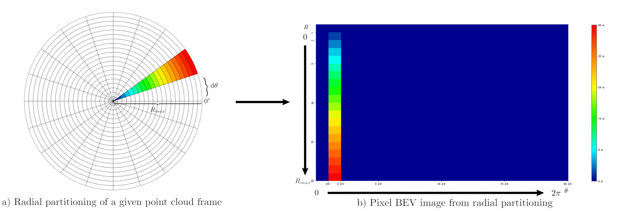
Figure 3. Process of BEV image generation. The partitioning of a point cloud is shown in (a), and the pixel image derived from the radial partitioning is shown in (b). Color of each pixel corresponds to a maximum point-to-plane distance according to the color bar on the right.

3.3. Retrieval

3.3.1. Database Construction and Update. The BEV pixel images generated from point cloud key-frames are used to search for possible candidates of loop closure. The pixel image, with N rows, M columns, and specific pixel values, corresponds to a N \( × \) M matrix. We here apply \( {L_{1}} \) normalization row-wise to the matrix, which yields a N \( × \) 1 matrix. The N \( × \) 1 matrix derived from each key-frame is then treated as a point in a N-dimensional space, which allows us to construct A k-D tree from these N-dimensional points. Using such data structure to conduct candidate searches can largely reduce computational time.

The construction process involves these key steps:

Choosing Splitting Axis: At each level of tree construction, the axis along which the data is split is determined. This decision can be based on criteria like alternating dimensions or selecting the axis with the highest variance.

Finding Splitting Value: After selecting the splitting axis, a splitting value is determined. This value is typically the median of the points projected onto the chosen axis.

Creating Subtrees: The data is divided into two subsets based on the splitting value. Subtrees are then created for each subset, and the construction process recurs on these subtrees.

To ensure the database’s relevance, a regular update mechanism is employed. Every 50 seconds, the k-D Tree database is refreshed by reconstructing the k-D Tree using the latest point cloud frame. The newly obtained N \( × \) 1 matrix is treated as a new N-dimensional point, and the k-D Tree is modified to incorporate this point while preserving its hierarchical structure.

The update procedure encompasses these main steps:

Finding Insertion Point: The existing k-D Tree is traversed to identify the appropriate leaf node where the new point should be inserted.

Expanding the Tree: Once the target leaf node is located, the k-D Tree is expanded to accommodate the new point. This ensures that the k-D Tree’s balance and structure are maintained.

3.3.2. Similarity Calculation. As each point cloud key-frame was previously encoded into a N-dimensional point from the k-D tree database, we search k (e.g., \( k=50 \) ) near neighbor point from the tree, each of which representing a possible loop closure candidate for each key-frame. We then calculate the similarity score between each candidate and the target key-frame. Here, we use the N \( × \) M matrix before encoding rather than the N \( × \) 1 matrix for calculation on both candidate and target to ensure the accuracy of loop closure detection. Since angular partitioning is applied to each point cloud key-frame, our proposed BEV descriptor is extremely sensitive to azimuthal changes. To ensure a robust detection method, we must have to apply column-wise shifting to the candidate matrix in consideration of azithumal angle variations. Since the matrix is N by M, we decide to shift the matrix for M times. \( {B_{o}} \) and \( {B_{k}} \) represent the matrix before and after each shift. To shift the matrix:

\( {B_{s}}(i,j)={B_{o}}(i,j+k),where k=0,1,2,...,M-1 \) (24)

For each shift, we calculate the similarity score between the shifted candidate matrix and the target matrix for once. For the calculation of the similarity score, we decide that a higher similarity score indicates a higher similarity between two BEV descriptors. Thus, the similarity function is:

\( S({B_{t}},B_{c}^{k})=1-\sum _{i=1,j=1}^{i=N,j=M} \frac{∣∣{B_{t}}(i,j)-B_{c}^{k}(i,j)∣∣}{N×M×{R_{max}}} \) (25)

where \( {B_{t}} \) represents the target descriptor and \( B_{c}^{k} \) represents the candidate descriptor after k shifts. Here, we mathematically derive the deviation of the shifted candidate descriptor from the target descriptor, and subtract the result from 1 to obtain a similarity score less than 1. After calculating similarity scores for all the shifted candidate descriptors, the highest similarity score will be assigned to the candidate. This assigned score will be used to compare with that of the other k candidates, and the final candidate \( {C_{L}} \) for loop closure is selected by highest assigned similarity score:

\( {C_{L}}=arg⁡max⁡S({B_{t}},{B_{c}}) \) (26)

3.3.3. ICP-based Geometric Verification. We use Iterative Closest Point (ICP) algorithm, a commonly-used algorithm for geometric alignment of two 3D point clouds, to geometrically verify whether a true loop closure has occur. The algorithm determines an optimal transformation that minimizes the disparities between corresponding points. However, unlike ICP used as an odometer, ICP used in our loop closure geometric verification finds the best transformation between the target key-frame and the candidate key-frame with the highest similarity score, rather than a target and a source point cloud. Apart from finding the translation vector and rotational matrix, we here compare the percentage of overlapping regions between two candidate point clouds ( \( {N_{o}} \) ) after transformation:

\( {N_{o}}=\frac{{N_{overlap}}}{{N_{sum}}}×100\% \) (27)

where \( {N_{overlap}} \) is number of overlapped points and \( {N_{sum}} \) is the number of total points, to a pre-set parameter \( σ \) (e.g., \( σ=50\% \) ) to determine whether a loop closure has occur. The percentage is obtained from dividing the numbers of overlapping points after transformation over the number of total points. If the percentage exceeds \( σ \) , a valid loop closure has occur between the two candidate point cloud frames.

3.3.4. Pose Graph Optimization. The pose graph consists of nodes that represent individual lidar point cloud scans. Two consecutive nodes, representing consecutive time steps, are linked by a transformation based on odometry information. This transformation includes a translation vector t and a rotational matrix R, typically obtained from LiDAR odometry.

The pose graph optimization process begins with an initial estimation of the poses of each LiDAR point cloud scan. Constraints are established between consecutive nodes based on odometry transformations. Given consecutive nodes i and j, the transformation \( {T_{ij }} \) from node i to node j is represented by the translation vector \( {t_{ij}} \) and the rotational matrix \( {R_{ij}} \) . The constraint equation is given by:

\( {T_{ij}}=[\begin{matrix}{R_{ij}} & {t_{ij}} \\ {0^{T}} & 1 \\ \end{matrix}] \) (28)

The goal of pose graph optimization is to minimize the discrepancy between the estimated poses and the constraints. The optimization objective can be defined as minimizing the sum of squared error terms between the estimated transformations and the constraint transformations:

\( min\sum _{i,j} ∥{T_{ij}}-T_{ij}^{est}∥_{F}^{2} \) (29)

where \( T_{ij}^{est} \) is the estimated transformation between nodes i and j.

Once a loop closure is detected between nodes i and k, a new constraint is added between these nodes. The transformation \( {T_{ik}} \) is obtained using ICP, yielding translation \( {t_{ik}} \) and rotation \( {R_{ik}} \) .

\( {T_{ik}}=[\begin{matrix}{R_{ik}} & {t_{ik}} \\ {0^{T}} & 1 \\ \end{matrix}] \) (30)

After adding loop closure constraints, the optimization objective is updated to include these new constraints. The optimization problem is solved again to refine the poses of all nodes, considering both odometer and loop closure constraints.

4. Experiment

Table 1. Experimental parameters

Table 2. LiDAR comparison from each dataset

Table 3. Selected dataset sequences for experiment

In this section, we evaluate our loop closure detection method on both open and private datasets with different scenarios (indoor and outdoor unstructured environment) to verify the effectiveness and adaptability of the method. In each experiment, we compare our method with state-of-the-art counterparts Scan Context [8] and VoxelMap proposed [19] by Yuan et al. on their default paramenters. All experiments are carried out on the same system with an Intel i5-12600kf @ 3.7 GHz with 32 GB memory.

4.1. Dataset Preparation

We use the KITTI odometry dataset and a private dataset for the validation of our method. The two datasets are chosen considering both LiDAR and scenario diversity to ensure the method’s adaptability under varying circumstances. Basic parameters of the two LiDARs used in both datasets are shown in Table 2. Characteristics of both datasets are summarized in Table 3.

1) KITTI odometry dataset: Developed by the Karlsruhe Institute of Technology (KIT) and the Toyota Technological Institute at Chicago (TTIC), KITTI odometry dataset provides a collection of synchronized sensor data in open urban environment, including grayscale stereo images, mechanical LiDAR scans, and accurate GPS/INS ground truth information. We evaluate our method on four sequences with the highest number of loop occurrence from the eleven sequences having the ground truth of pose (from 00 to 10), namely KITTI00, KITTI02, KITTI05, and KITTI08. While the other three sequences have loops in the same direction, only KITTI08 has reverse loops. LiDAR data from the dataset is obtained from a Velodyne 64-ray mechanical spinning LiDAR.

2) Private Dataset: We select four sequences from our dataset: one indoor and three outdoor sequences. The dataset was collected around summer of the year 2023, originating from a typical residential quarter within Minhang district of Shanghai. LiDAR and IMU data from the dataset are collected on a pre-built robotic vehicle as shown in Figure 4.(b), equipped with a HEXMAN MARK-2 chassis, a Livox Mid-360 solid state LiDAR and a built-in IMU. The indoor sequence, ID2, has a total length of 621 m, is recorded at the underground parking lot of the residential quarter. The outdoor sequence, OD2, has a total length of 957 m, is recorded at the interior of the residential quarter; the rest two outdoor sequences, having a total length of 1423 m and 1955 m respectively, are both recorded at the peripheral area of the residential quarter. The trajectories of all sequences are shown in Figure 5.

We set the experimental parameters as shown in Table 1. For KITTI dataset, we evaluate the performance of our proposed method on loop closure detection by the precision-recall curve, compared with Scan Context, another state-of-art point cloud descriptor. Then, given the constraints from detected loop closures, accuracies of the trajectories before and after pose graph optimization will be compared. Our private dataset will not be evaluated through the above two measures due to the lack of ground truth; it will rather serve as an additional validation of the adaptability of our proposed method under varying LiDAR types and environments.

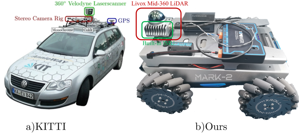
Figure 4. Recording platform with sensors (a) from KITTI dataset [20] and (b) our private dataset

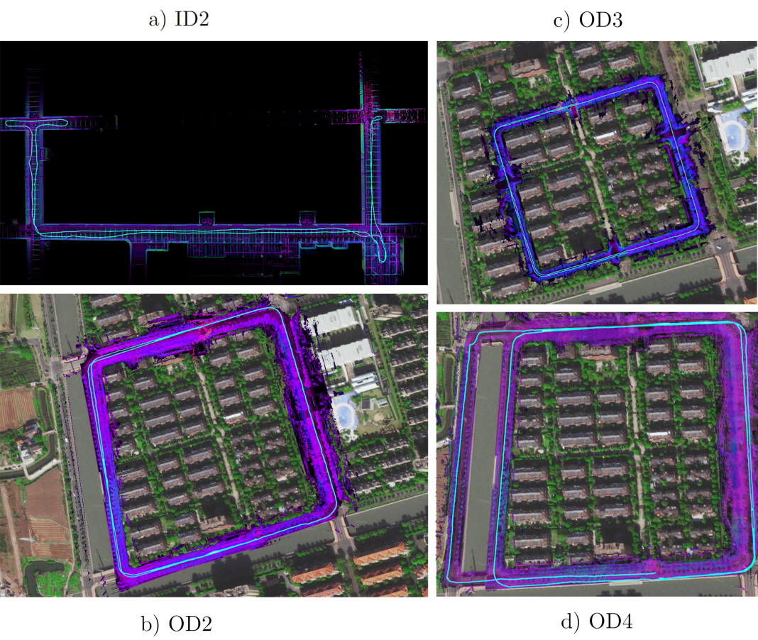
Figure 5. Trajectories of the four sequences, aligned with their corresponding point cloud and satellite image. In (a), the path of sequence ID2 is a semi-loop with its reverse loop. In (b) and (c), the paths of sequences OD2 and OD3 are all full loops. In (d), the path of sequence OD4 consists of a smaller loop and a larger loop.

4.2. Precision Recall Evaluation

The precision-recall curves for both our proposed BEV descriptor and Scan Context on KITTI odometry sequences are illustrated in Figure 7. From the results, our method outperforms Scan Context in most sequences. Both methods have a similar curve shape, yet our method has a slight increase in recall rate in all sequences except KITTI02. Like our method, Scan Context is sensitive to azimuthal variances; however, it mainly relies on vertical structure information as its bin encoding uses a maximum height, limiting its performance when the vertical height in the surrounding varies a little. In comparison, our approach relies on plane projection and replaces maximum height with maximum point-to-plane distance. This allows more variances in vertical structure and increases robustness of the descriptor against changes in pitch angle, ultimately enhancing its overall performance. According to Figure 6, the performance of our method on sequence KITTI02 is poorer than on any other sequence, probably due to sparse structures or occlusion issue of the loop closure in the scene [9] [21]. An example scene in the sequence is shown in Figure 6.

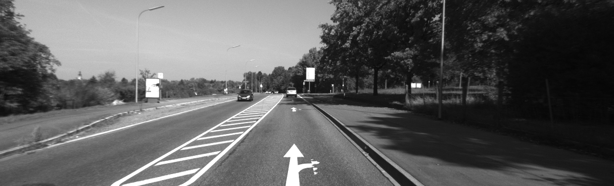
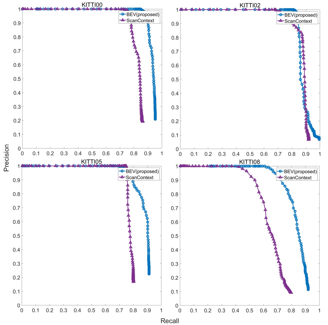
Figure 7. Precision-recall curves on four KITTI odometry sequences.

To further compare the detection performance, we calculate the F1 scores on both methods over four sequences. The results in Table 4, consistent with the precision-recall curves, shows a higher score on our method than on Scan Context. In addition, our method improves the most over sequence KITTI08, indicating our method can effectively detect reverse loop closures with higher robustness to azimuthal changes.

Table 4. F1 scores over four KITTI odometry sequences

4.3. Trajectory Accuracy Evaluation

To demonstrate the improvement of mapping quality through our loop closure detection method, we use VoxelMap [19], a high accuracy odometer, to generate the trajectories of the four KITTI sequences. In contrast, we further use the constraints from detected loop closures in the sequences to correct the trajectories. As shown in Figure 8, we compare the original trajectories of four sequences mapped by VoxelMap, with the trajectories after correction by our method. The distance error between each trajectory and the ground truth is then calculated. From the results, the accuracies of the trajectories after correction by our method has notably improved. No signs of huge drifts or deviations from the original trajectories are shown in results, hence indicating that loop closures in the four sequences can be accurately detected through our proposed method and utilized to improve the quality and precision of long-term mapping. It is worth noticing that in sequence KITTI02, the start of the trajectory after correction had experience a comparably large drift, probably due to the sparse structures on the highway scene as key points extracted in such scenes are scarce. This finding of a relatively poor performance on KITTI02 is consistent with the results in previous section.

The average Root Mean Square Error (RMSE) of each trajectories is summarized in Table 5. The trajectories after correction by our approach produce a reduced average RMSE. The average RMSE of KITTI02 trajectory after correction decreases less significantly than that of the other three sequences. Therefore, our loop closure detection method can be integrated into SLAM context to provide accurate loop closure detection under varying conditions.

Table 5. Average RMSE of trajectories before and after correction Unit: m

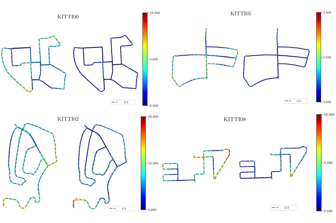
Figure 8. Trajectories (left) generated by VoxelMap compared to trajectories (right) after correction by our approach. The color bar on the right indicates distance error between the generated trajectory and the ground truth. Unit: m

4.4. Runtime Evaluation

We record the computation time on KITTI05 for our method and Scan Context. For Scan Context, we test with its provided Python API with the default parameter. As shown in Figure 9, both methods’ computational time increases with the number of key-frames, possibly due to the construction of k-d tree for retrieval in both methods. Overall, our method has a more consistent computational time over time and a less computational time per frame than Scan Context. The difference on how we test the two methods (generically on ours and using an API for Scan Context) might account for our superiority, but an average computational time of less than 100 ms per frame is sufficient to verify our proposed descriptor as an efficient descriptor for loop closure detection.

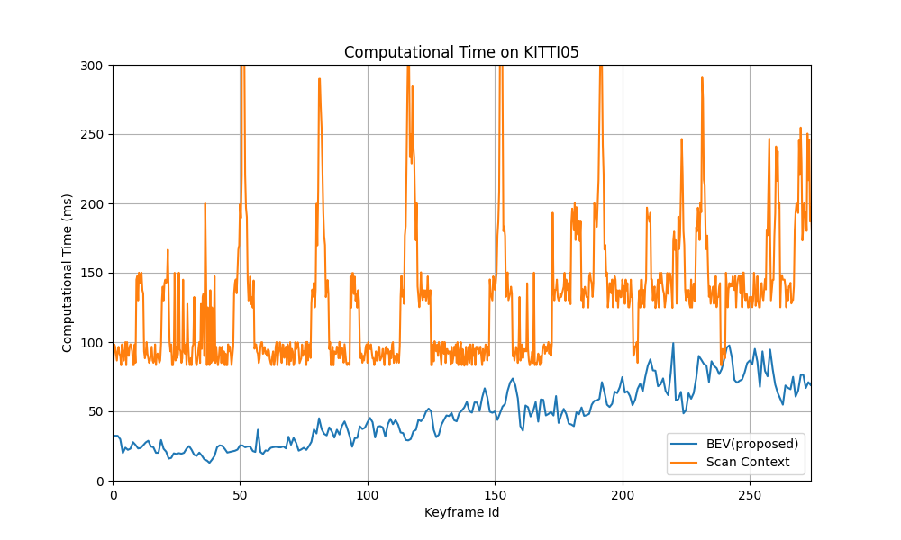
Figure 9. Compuational time on KITTI05 of our proposed BEV method

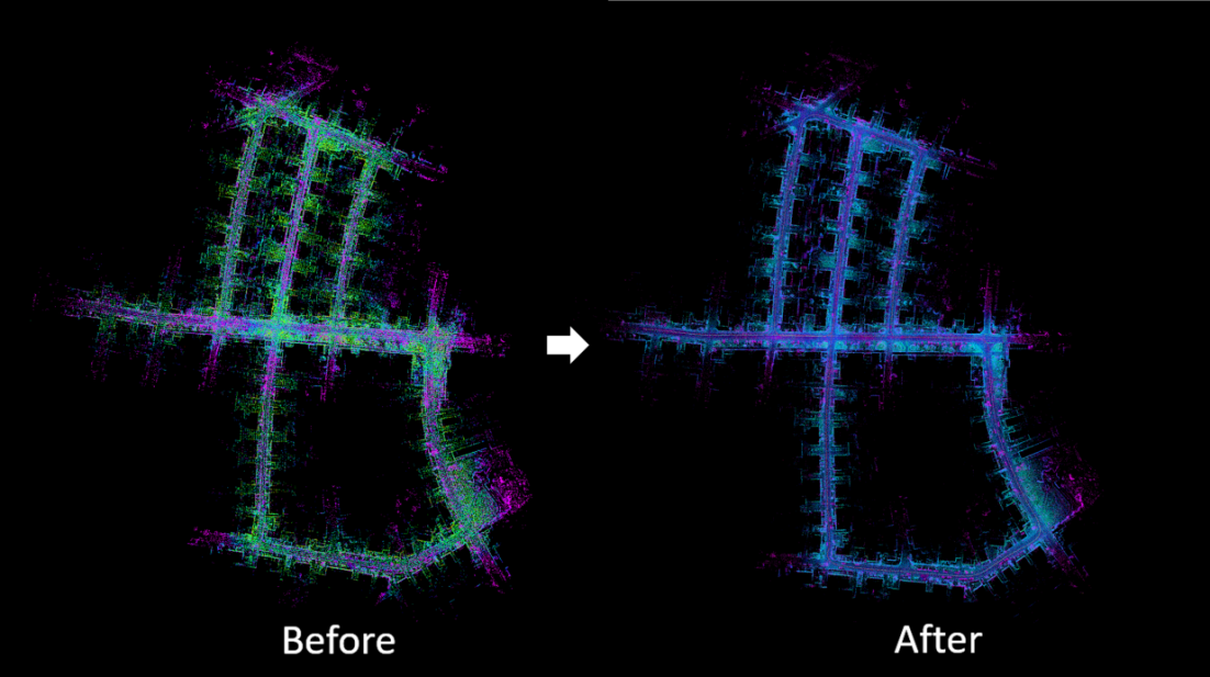
Figure 10. KITTI05 point cloud map before and after correction by our approach

5. Conclusion

This paper proposes a adaptive and robust BEV point cloud descriptor. An effective BEV image generation process based on plane detection and projection and space partition is proposed to extract and preserve geometric information from each point cloud key-frames. Through radial and azimuthal partition, our descriptor exhibits resilience against changes in azimuthal and pitch angles. To speed up the querying and retrieval process, we further construct a k-d Tree database for searching possible loop closure candidates and compute similarity scores between the candidates. Compared with Scan Context, a state-of-art global descriptors, our method not only outperforms Scan Context in KITTI dataset but also demonstrate a great robustness and adaptability to both outdoor and indoor environment and to different, less costly LiDAR types.

References

[1]. Mathieu Labbe and Fran ̧cois Michaud. Online global loop closure detection for large-scale multi-session graph-based slam. In 2014 IEEE/RSJ International Conference on Intelligent Robots and Systems, pages 2661–2666. IEEE, 2014.
[2]. Saba Arshad and Gon-Woo Kim. Role of deep learning in loop closure detection for visual and lidar slam: A survey. Sensors, 21(4):1243, 2021.
[3]. Mathieu Labbe and Fran ̧cois Michaud. Online global loop closure detection for large-scale multi-session graph-based slam. In 2014 IEEE/RSJ International Conference on Intelligent Robots and Systems, pages 2661–2666. IEEE, 2014.
[4]. Ben Glocker, Jamie Shotton, Antonio Criminisi, and Shahram Izadi. Real-time rgb-d camera relocalization via randomized ferns for keyframe encoding. IEEE transactions on visualization and computer graphics, 21(5):571–583, 2014.
[5]. Andrés C Jiménez, Vicente García-Díaz, and Sandro Bolaños. A decentralized framework for multi-agent robotic systems. Sensors, 18(2):417, 2018.
[6]. Stephanie Lowry, Niko S ̈underhauf, Paul Newman, John J Leonard, David Cox, Peter Corke, and Michael J Milford. Visual place recognition: A survey. ieee transactions on robotics, 32(1):1–19, 2015.
[7]. Wei Xu, Yixi Cai, Dongjiao He, Jiarong Lin, and Fu Zhang. Fast-lio2: Fast direct lidar-inertial odometry. IEEE Transactions on Robotics, 38(4):2053–2073, 2022.
[8]. Giseop Kim and Ayoung Kim. Scan context: Egocentric spatial descriptor for place recognition within 3d point cloud map. In 2018 IEEE/RSJ International Conference on Intelligent Robots and Systems (IROS), pages 4802–4809. IEEE, 2018.
[9]. Chongjian Yuan, Jiarong Lin, Zuhao Zou, Xiaoping Hong, and Fu Zhang. Std: Stable triangle descriptor for 3d place recognition. In 2023 IEEE International Conference on Robotics and Automation (ICRA), pages 1897–1903. IEEE, 2023.
[10]. Huan Yin, Xuecheng Xu, Sha Lu, Xieyuanli Chen, Rong Xiong, Shaojie Shen, Cyrill Stachniss, and Yue Wang. A survey on global lidar localization. arXiv preprint arXiv:2302.07433, 2023.
[11]. Mark Cummins and Paul Newman. Fab-map: Probabilistic localization and mapping in the space of appearance. The International journal of robotics research, 27(6):647–665, 2008.
[12]. Adrien Angeli, David Filliat, St ́ephane Doncieux, and Jean-Arcady Meyer. Fast and incremental method for loop-closure detection using bags of visual words. IEEE transactions on robotics, 24(5):1027–1037, 2008.
[13]. Dorian Gálvez-López and Juan D Tardos. Bags of binary words for fast place recognition in image sequences. IEEE Transactions on Robotics, 28(5):1188–1197, 2012.
[14]. Christoffer Valgren and Achim J Lilienthal. Sift, surf and seasons: Long-term outdoor localization using local features. In 3rd European conference on mobile robots, ECMR’07, Freiburg, Germany, September 19-21, 2007, pages 253–258, 2007.
[15]. Michael J Milford and Gordon F Wyeth. Seqslam: Visual route-based navigation for sunny summer days and stormy winter nights. In 2012 IEEE international conference on robotics and automation, pages 1643–1649. IEEE, 2012.
[16]. Fei Han, Xue Yang, Yiming Deng, Mark Rentschler, Dejun Yang, and Hao Zhang. Sral: Shared representative appearance learning for long-term visual place recognition. IEEE Robotics and Automation Letters, 2(2):1172–1179, 2017.
[17]. Renaud Dubé, Daniel Dugas, Elena Stumm, Juan Nieto, Roland Siegwart, and Cesar Cadena. Segmatch: Segment based place recognition in 3d point clouds. In 2017 IEEE International Conference on Robotics and Automation (ICRA), pages 5266–5272. IEE
[18]. John Crassidis and F Markley. Attitude estimation using modified rodrigues parameters. In NASA Conference Publication, pages 71–86. NASA, 1996.
[19]. Chongjian Yuan, Wei Xu, Xiyuan Liu, Xiaoping Hong, and Fu Zhang. Efficient and probabilistic adaptive voxel mapping for accurate online lidar odometry. IEEE Robotics and Automation Letters, 7(3):8518–8525, 2022.
[20]. Andreas Geiger, Philip Lenz, and Raquel Urtasun. Are we ready for autonomous driving? the kitti vision benchmark suite. In 2012 IEEE conference on computer vision and pattern recognition pages 3354–3361. IEEE, 2012.
[21]. Gang Wang, Xiaomeng Wei, Yu Chen, Tongzhou Zhang, Minghui Hou, and Zhaohan Liu. A multi-channel descriptor for lidar-based loop closure detection and its application. Remote Sensing, 14(22):5877, 2
Cite this article
Qu,A. (2024). Adaptive bird's eye view description for long-term mapping and loop closure in 3D point clouds. Applied and Computational Engineering,73,77-93.
Data availability
The datasets used and/or analyzed during the current study will be available from the authors upon reasonable request.
Disclaimer/Publisher's Note
The statements, opinions and data contained in all publications are solely those of the individual author(s) and contributor(s) and not of EWA Publishing and/or the editor(s). EWA Publishing and/or the editor(s) disclaim responsibility for any injury to people or property resulting from any ideas, methods, instructions or products referred to in the content.
About volume
Volume title: Proceedings of the 2nd International Conference on Software Engineering and Machine Learning
© 2024 by the author(s). Licensee EWA Publishing, Oxford, UK. This article is an open access article distributed under the terms and
conditions of the Creative Commons Attribution (CC BY) license. Authors who
publish this series agree to the following terms:
1. Authors retain copyright and grant the series right of first publication with the work simultaneously licensed under a Creative Commons
Attribution License that allows others to share the work with an acknowledgment of the work's authorship and initial publication in this
series.
2. Authors are able to enter into separate, additional contractual arrangements for the non-exclusive distribution of the series's published
version of the work (e.g., post it to an institutional repository or publish it in a book), with an acknowledgment of its initial
publication in this series.
3. Authors are permitted and encouraged to post their work online (e.g., in institutional repositories or on their website) prior to and
during the submission process, as it can lead to productive exchanges, as well as earlier and greater citation of published work (See
Open access policy for details).