1. Introduction

Computers play a significant role in human society. People do all kinds of work with their computers, one of which is to process images and pictures from the real world. Computer vision is about how machines “see” and process what they see. In fields like auto driving, the auto needs to analyze and build a model of the surrounding environment in order to stay in the lane and avoid any possible crashes. The “analyze” procedure includes image processing, which extracts information from the images collected by the camera. Moreover, the auto needs to recognize which part of the image is the road, pedestrians, other automobiles, etc., and behave based on the recognition result. There is a subject called semantic segmentation to handle this recognition task.

Semantic segmentation is based on another technology named machine learning. Machines can learn the strategy to deal with all kinds of tasks, and recognizing objects is one of them.

One way for machines to learn is by feeding a large amount of data with labels and rewarding the agent if it gets the correct label from the data or punishing the agent if the label is wrong. The agent would adjust the strategy to maximize the correct rate and get as many rewards as possible. When the training is complete, the agent has learned how to label new and unseen data with high accuracy. This is called supervised learning and is very common in applications like handwriting recognition, optical character recognition, junk mail detection, and many others.

Although machines can automatically learn the strategy when given proper data, we must still help them build the learning model. This is about “how to learn strategies” rather than “how to solve problems.” One widely applied model is the neural network, inspired by the human’s neural system connection. Superficial nodes, called “neurons” in the neural network, connect with each other like neurons do in a living creature. Data flows through the network and gets processed in each layer (Forward Propagation) until they reach the last layer and get the answer.

Deep learning is a branch of machine learning based on the neural network. The word “deep” in deep learning usually means multiple layers in the network. Earlier works showed that linear perceptron cannot be a universal classifier, while a network with a non-polynomial activation function and a hidden layer of infinite nodes can. As we usually lack the resources to store and train on an infinite network, a more practical way is to replace the hidden layer with multiple layers of finite nodes. It has been applied in many fields, like computer vision.

Semantic segmentation aims to segment the image and classify each part of an image. That is to say, to assign different labels to every pixel of an image so that pixels of the same label share some familiar visual characters. Back to the auto driving example, the auto needs to process every frame as fast and accurately as possible. If the segmentation takes too long, a car crash may occur before the auto realizes what is wrong. If the segmentation recognizes something falsely, the auto may run into a dead end while still thinking itself in the lane. The most advanced segmentation algorithms are all based on deep learning, and here, we would like to investigate some of them and see how they perform on relatively small datasets.

2. Related Works

2.1. Multilayer Perceptron

A Multilayer Perceptron (MLP) is a type of feedforward neural network that consists of fully connected neurons, each employing a nonlinear activation function. Typically, an MLP is structured with at least three layers: an input layer, one or more hidden layers, and an output layer, where each layer is fully interconnected with its preceding and subsequent layers. This means that every node within one layer connects with every node in the adjacent layers.

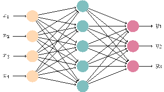
Figure 1. MLP structure

In this architecture, each node is assigned a specific value, and every connection between nodes is associated with a weight. The values of a given layer are computed based on the values of the preceding layer and the weights of the connections between them. For computational purposes, the values of a layer can be represented as a vector \( {v_{i}} \) , and the connection weights as a weight matrix \( {W_{i}} \) . Consequently, the values for the next layer are derived through matrix multiplication, expressed as \( v_{i+1}^{ \prime }={W_{i}}\cdot {v_{i}} \) .

Following this matrix multiplication, the resultant values must undergo a process termed “activation” via an activation function. Drawing from linear algebra, it is understood that the multiplication of a vector by several matrices is equivalent to multiplying the vector by the product of these matrices. Without a nonlinear activation function, an MLP would regress to the functionality of a single-layer perceptron.[1] The inclusion of a nonlinear activation function is therefore essential for the MLP’s ability to classify nonlinear data. Commonly utilized activation functions include the sigmoid function \( σ(z) \) , the hyperbolic tangent function \( tanh{(z)} \) , and the rectified linear unit (ReLU) function \( relu(z) \) . This non-linearity is crucial to prevent the MLP from simplifying into a linear model, enabling it to tackle complex classification tasks effectively.

\( σ(z)=\frac{1}{1+{e^{-z}}} \)

\( tanh{(z)}=\frac{{e^{z}}-{e^{-z}}}{{e^{z}}+{e^{-z}}} \)

\( relu(z)=max{(0,z)} \)

The real value of a layer is \( {v_{i+1}}=ϕ(v_{i+1}^{ \prime }) \) , where \( v_{i+1}^{ \prime } \) is the result of the matrix multiplication. The values in the output layer are activated by another function, softmax, to normalize the values and imply the probability that the input data belongs to each class. The maximum value suggests that the input will most likely belong to this class.

The feedforward network is commonly trained by the backpropagation method. Each time the network gives a prediction, it will adjust the weights of each connection based on the error between the predicted probability and the reference probability. We denote the error of the \( j \) -th node from the output layer in the \( n \) -th input data by \( e_{j}^{n} \) . The overall error is

\( {e^{n}}=\frac{1}{2}\sum _{j}{(e_{j}^{n})^{2}} \)

Using gradient descent, the change in each weight \( {w_{ij}} \) is

\( Δw_{ji}^{n}=-η\frac{∂{e^{n}}}{∂v_{j}^{n}}y_{i}^{n} \)

where \( y_{i}^{n} \) is the \( i \) -th output of the previous neuron on the \( n \) -th data. \( η \) is the learning rate and has to be selected wisely. A small learning rate may cause the algorithm to be slow, as more steps are needed to converge, and a large learning rate may cause the weight to oscillate, as the weight may step over the converging point.

The derivative of an output layer node can be simplified to

\( -\frac{∂{e^{n}}}{∂v_{j}^{n}}=e_{j}^{n}{ϕ^{ \prime }}(v_{j}^{n}) \)

where \( {ϕ^{ \prime }} \) is the derivative of the activation function.

The derivative of a hidden layer node is

\( -\frac{∂{e^{n}}}{∂v_{j}^{n}}={ϕ^{ \prime }}(v_{j}^{n})\sum _{k}-\frac{∂{e^{n}}}{∂v_{k}^{n}}w_{kj}^{n} \)

This depends on the weight change of the \( k \) -th nodes, which represent the output layer. So, to change the hidden layer weights, the output layer weights change according to the derivative of the activation function. Thus, this algorithm represents a backpropagation of the activation function.[2]

2.2. Convolutional Neural Network

The Convolutional Neural Network (CNN) is a type of feedforward network that distinguishes itself by incorporating at least one convolutional layer within its hidden layers. This layer, along with fully connected layers akin to those found in Multilayer Perceptrons (MLPs) and pooling layers to downscale data dimensions, allows CNNs to efficiently process the two-dimensional structure of input data. Consequently, CNNs exhibit superior performance in tasks such as image and voice recognition when compared to other deep learning models. The inspiration for this architecture stems from the neural connections within the animal visual cortex, where individual neurons respond to stimuli within a restricted area, with the perceptual fields of various neurons overlapping to encompass the entire visual field.

In the convolutional layer, a set of feature maps is generated by applying a convolution kernel to the input image. This operation involves an element-wise multiplication followed by a summation, effectively reducing an area of the kernel’s size in the input to a single numerical value. Consequently, the dimensional footprint of the matrix diminishes with each pass through a convolutional layer. A layer of Rectified Linear Units (ReLU) is commonly employed as the activation function to introduce non-linearity.

Although fully connected feedforward neural networks can be used to learn features and classify data, this architecture is generally impractical for larger inputs like high-resolution images, as the network would have too many neurons and weights. Convolution reduces the number of free parameters, allowing the network to be deeper.[3]

The input image, potentially vast in size, often contains adjacent pixels that are similar and likely depict the same object. To abstract a more generalized representation of the image, pooling layers are utilized to condense the outputs of neuron clusters at one layer into a single neuron in the subsequent layer. Max pooling, the most prevalent form of pooling, reduces data volume by 75% by selecting the maximum value from every \( 2×2 \) pixel area. Concluding the process, several fully connected layers assume the role of classifying the image, employing a methodology similar to that of the MLP. This structured approach enables CNNs to efficiently handle complex pattern recognition tasks, leveraging their unique architecture to achieve remarkable performance in various applications.

3. Methods

3.1. Fully Convolutional Network

The Fully Convolutional Network (FCN), developed by Jonathan Long, Evan Shelhamer, and Trevor Darrell at the University of California, Berkeley, represents a significant advancement in the field of semantic segmentation. An FCN is characterized by its exclusive reliance on convolutional operations, which may include subsampling or upsampling, to process input data. This architecture distinguishes itself from conventional Convolutional Neural Networks (CNNs) by omitting fully connected layers. However, it is noteworthy that fully connected layers can be conceptualized as convolutions with kernels spanning the entire input area. Consequently, a CNN can be transformed into an FCN through a process of fine-tuning, facilitating a seamless transition that leverages the strengths of convolutional processing for semantic segmentation tasks.

The sizes of fully connected layers are pre-defined, forcing a CNN model to only accept fixed-size images. The FCN removes these fully connected layers and thus takes images of arbitrary sizes. Moreover, the FCN utilizes \( 1×1 \) convolutions and trans-convolutions to restore the original size of the image, making an end-to-end pixel-to-pixel prediction.[4]

The Fully Convolutional Network (FCN) integrates information from earlier layers to achieve a comprehensive understanding of the image. This approach ensures the retention of finer details, enabling the generation of precise segmentation boundaries. Through this method, FCNs effectively balance the need for a global perspective with the preservation of local nuances, facilitating accurate and detailed semantic segmentation.

3.1.1. The architecture FCN. The FCN starts by convolutionizing existing classification architectures. Many networks, including AlexNet, VGG 16, and GoogLeNet, can be used as the backbone of FCN. The VGG 16 performs best among these networks, and here we will review the architecture of VGG 16 first.The input layer takes a colorful image in the size of \( 224×224×3 \) .

• Block 1

Convolutional layer fc1_1 and fc1_2. Each layer convolutes the result from the last layer with 64 \( 3×3 \) kernels to produce a \( 224×224×64 \) feature map.

Max pooling layer pool1. It downsamples the image by \( 2×2 \) and produces a \( 112×112×64 \) feature map.

• Block 2

Convolutional layer fc2_1 and fc2_2. They are similar to convolutional layers 1 and 2 but enlarge the number of kernels to 128 and produce a \( 112×112×128 \) feature map.

Max pooling layer pool2. It downsamples the image by \( 2×2 \) and produces a \( 56×56×128 \) feature map.

• Block 3

Convolutional layer fc3_1 and fc3_2. They again enlarge the number of kernels to 256 and produce a \( 56×56×256 \) feature map.

Max pooling layer pool3. It downsamples the image by \( 2×2 \) and produces a \( 28×28×256 \) feature map.

• Block 4

Convolutional layer fc4_1 and fc4_2. They further enlarge the number of kernels to 512 and produce a \( 28×28×512 \) feature map.

Max pooling layer pool4. It downsamples the image by \( 2×2 \) and produces a \( 14×14×512 \) feature map.

• Block 5

Convolutional layer fc5_1 and fc5_2. This time, they keep the number of kernels 512 unchanged and produce a \( 14×14×512 \) feature map.

Max pooling layer pool5. It downsamples the image by \( 2×2 \) and produces a \( 7×7×512 \) feature map.

• Fully connected layers

Fully connected layer 1. It takes \( 7×7×512 \) neurons and outputs 4096 neurons.

Fully connected layer 2. It takes 4096 neurons and outputs 4096 neurons.

Fully connected layer 3. It takes 4096 neurons and outputs 1000 neurons.

Every convolutional layer and fully connected layer is activated by a ReLU function. The last layer is normalized by SoftMax.

The FCN discards the final classification layer and replaces all fully connected layers with convolutional layers. Then, append a \( 1×1 \) convolutional layer with as many channels as classes, followed by a deconvolution layer to upsample the output back to the size of the original image. The convolutional layer can take input in any size. Suppose that the image is \( h×w \) , and the number of classes is \( n \) .

• Convolutional layer fc6. Using kernels of \( 7×7 \) and dropout, it produces a \( \frac{h}{32}×\frac{w}{32}×4096 \) feature map.

• Convolutional layer fc7. Using kernels of \( 1×1 \) and dropout, it produces a \( \frac{h}{32}×\frac{w}{32}×4096 \) feature map.

• Convolutional layer fc8. Using kernels of \( 1×1 \) , it produces a \( \frac{h}{32}×\frac{w}{32}×n \) feature map.

• Transpose convolutional layer. In order to restore the original size, the feature map is upsampled by 32 times and produces a \( h×w×n \) feature map.

3.1.2. The variations of FCN. In the network architecture previously described, the feature map is upsampled by a factor of 32, leading to its designation as FCN-32. However, directly upsampling by a factor of 32 often results in diminished accuracy. A proposed solution to this issue involves the integration of outputs from different convolutional layers. Instead of a singular 32-fold upsampling, the process begins with the result of the pool5 layer being upsampled by a factor of two, aligning its dimensions with those of the pool4 layer’s result. These results are then combined and subsequently upsampled by a factor of 16, a technique referred to as FCN-16.

Advancing this concept, the combined output from the FCN-16 stage is upsampled once more by a factor of two, matching the dimensions of the pool3 layer’s result. Following another summation, this output is upsampled by a factor of eight. This iterative refinement culminates in FCN-8, which stands as the most precise iteration of the Fully Convolutional Network, effectively balancing resolution enhancement with the preservation of segmentation accuracy.

3.2. The DeepLab family

DeepLab, a novel model family within the realm of semantic segmentation, was developed by Liang-Chieh Chen, alongside his colleagues at UCLA and Google. This team has achieved notable success in visual recognition, representation, and deep learning. Originating from the Fully Convolutional Network (FCN) concept, the DeepLab family has introduced four iterations – versions 1, 2, 3, and 3+ – between 2015 and 2018. Each version built upon its predecessor, incorporating advancements from recent image classification innovations to enhance semantic segmentation and stimulate further research in the domain. These developments underscore the evolution of deep convolutional neural networks in semantic segmentation.

3.2.1. DeepLabv1. DeepLab first came out in 2016[5]. DeepLabv1 amalgamates two established methodologies: Deep Convolutional Neural Networks (DCNNs) and fully connected Conditional Random Fields (CRFs). Semantic segmentation networks, evolving from image classification networks, typically employ a backbone network that has proven effective in image classification tasks. For instance, as early as 2014, the VGG network, utilizing \( 3×3 \) convolution kernels, surpassed AlexNet, establishing itself as the premier solution for image classification. Both DeepLabv1 and FCN leverage the VGG-16 as their backbone network for feature extraction and granular classification.

A pivotal innovation in DeepLabv1 is the introduction of dilated convolutions. This technique involves expanding the convolutional filters’ field of view through a dilation rate[6], thereby broadening the contextual scope considered by the filter. This approach mimics an upsampling operation but maintains the same parameter count, thereby avoiding increased computational costs. It achieves this by omitting pixels between the targets of the upsampled filter. The application of atrous convolution allows the network to manage the reduced spatial resolution inherent in deep feature extractors while producing a larger output matrix and circumventing the need for aggressive upsampling. Although the output from DCNNs constitutes a segmentation map, the precise localization of features necessitates further refinement, achieved through the application of fully connected CRFs to enhance performance.

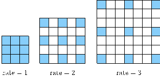
Figure 2. Atrous convolution with a \( 3×3 \) kernel and different rates. Blocks in color are taken into consideration.

Conditional Random Fields (CRFs) are composed of interconnected nodes, each assigned a label influenced by its immediate neighbors. They are frequently employed to mitigate noise and accentuate boundaries within noisy segmentation maps. By applying CRFs iteratively to the output of Deep Convolutional Neural Networks (DCNNs), the segmentation map becomes progressively refined, achieving clearer boundaries near object edges. In the context of DeepLabv1, approximately ten iterations of CRF application are sufficient to produce a segmentation map of adequate accuracy. However, it’s important to recognize CRFs as a post-processing technique; this architecture does not support end-to-end and real-time prediction capabilities.

3.2.2. DeepLabv2. The second iteration of DeepLab, introduced in 2017 by the original authors, marked a significant enhancement by substituting the VGG backbone with ResNet and incorporating Atrous Spatial Pyramid Pooling (ASPP) within the convolutional layers.

Long before the advent of deep learning, spatial pyramids were a cornerstone algorithm in computer vision, serving as a fundamental technique for numerous algorithms, such as SIFT, to maintain consistent scale. The introduction of the Spatial Pyramid Pooling (SPP) network brought the concept of spatial pyramids into convolutional networks, with DeepLabv2 advancing this by introducing an atrous variant of the SPP module.

The SPP module enables the network to encapsulate features of varying scales into fixed-size feature maps, somewhat akin to the “bag of words” approach. However, instead of merely aggregating elements, it involves assigning elements within new feature vectors in varying proportions based on their scale. For instance, one eigenvalue may represent the global scale, two eigenvalues the larger scale, and three eigenvalues the smaller scale. Consequently, a fixed-size feature map comprising six values is obtained. In the actual ASPP module, as illustrated, four different scales are defined by varying atrous rates (6, 12, 18, 24), allowing for a comprehensive encoding of features across multiple scales.[7]

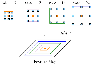
Figure 3. Atrous Spatial Pyramid Pooling (ASPP)

In the architectures of FCN and DeepLabv1, the input dimension is constrained to \( 224×224 \) to align with the predetermined connectivity of the fully convolutional layer, which is \( 28×28×1024 \) . The introduction of the Spatial Pyramid Pooling (SPP) module enables our network to accommodate inputs of varied sizes without necessitating modifications to the fully convolutional layer. This flexibility is partly due to the atrous convolution employed by the SPP module, which additionally confers the benefits of an expanded field of view and reduced computational demand. A notable distinction between versions 1 and 2 of DeepLab is the implementation of a new multiscale structure. Unlike its predecessor, DeepLabv2 circumvents the need to process computational features at different scales by applying parallel processing to images scaled at 1.0, 0.75, and 0.5, thereby facilitating multiscale feature fusion. The efficacy of this design is debatable, as executing identical computations thrice inevitably prolongs both inference and training times. However, its effectiveness in enhancing performance on the PASCAL dataset is unequivocal, underscoring its value in improving semantic segmentation outcomes.

3.2.3. DeepLabv3. The implementation of atrous convolution and spatial pyramid pooling significantly contributed to the successes of DeepLabv1 and v2, prompting the authors to further investigate this approach, particularly focusing on the Atrous Spatial Pyramid Pooling (ASPP) module. DeepLabv3 continues to utilize the ResNet backbone. Unlike in v2, where ASPP amalgamated features of four different scales into a single fixed-size feature, the unique characteristics of atrous convolution presented challenges in capturing both minuscule local features, such as tiny edges, and extensive global features.

To encompass a broader spectrum of information, DeepLabv3 introduced a redesign of the ASPP module to incorporate a separate global image pooling channel for global features. This is then combined with the ASPP via a 1x1 convolutional cascade, enabling the network to utilize fine-grained details. Additionally, the ASPP module was enhanced by integrating batch normalization post-convolution and pre-ReLU.[8]

The approach to multi-scale methods in DeepLabv3 also deviates from that of DeepLabv2. Recognizing the inefficiencies in the training process of DeepLabv2, the authors opted to apply multi-scale techniques during inference instead. Consequently, during training, the network employs only the original image scale rather than three. At inference, the network processes the input image at six different scales – 0.5, 0.75, 1.0, 1.25, 1.5, and 1.75 – averaging the outputs to refine the results.

DeepLabv3’s advancements in benchmarking metrics signify a point of optimization where adding Conditional Random Fields (CRF) post-processing steps became redundant. As a result, CRF was omitted in DeepLabv3 and subsequent versions. Employing multi-scale and flip techniques, alongside the generation of expansive feature maps through reduced output strides, effectively mitigates prediction uncertainties, enhancing the network’s final output accuracy.

3.2.4. DeepLabv3+. DeepLabv3+ is the most up-to-date version of the DeepLab family, presented in 2018[9].

Encoding has become a foundational concept in semantic segmentation, with prominent frameworks such as FCN, U-Net, and E-Net embracing this strategy. These models initially leverage a backbone network to compress the image into a compact feature vector, followed by the employment of a ConvolutionTranspose layer to develop a decoder network that upsamples the features. Convolution transpose serves as the inverse of convolution, distributing values from a singular point across a broader area rather than aggregating multiple inputs into one. The decoder’s objective is to devise a methodology for reconstructing the information lost during the encoding phase. However, in DeepLabv1 and v2, the authors critiqued the reliance on the encoder-decoder paradigm, positing that atrous convolution, with its capability for high-resolution processing, could similarly facilitate upsampling effects while minimizing information loss. Despite this, the decoder structure, particularly convolution transpose, remains prevalent in other network designs due to its straightforward implementation. Consequently, DeepLabv3+ assimilates a nuanced comprehension of the encoder-decoder framework to further enhance model performance, bridging the gap between theoretical critique and practical application in the evolution of semantic segmentation technologies.

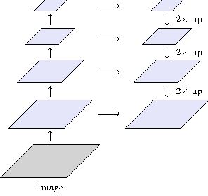
Figure 4. The Encoder-Decoder structure in DeepLabv3+

The encoder component of DeepLabv3+ is derived from the original DeepLabv3 network, comprising both the backbone DCNN and the Atrous Spatial Pyramid Pooling (ASPP) module. Inputs to the decoder include the output from the ASPP and an intermediate feature output from the backbone network, with the decoder employing convolution and bilinear upsampling to incrementally enhance the resolution of the output by a factor of eight. Interestingly, the DeepLabv3 study revealed that incorporating global pooling (image-level feature fusion) within the ASPP module, when used alongside the decoder, actually detracted from the model’s performance on the Cityscapes dataset. This observation might indicate that the functional fusion strategies employed in DeepLab have reached a point of saturation, where additional integrations fail to contribute to performance improvements. It suggests the possibility that the network architecture could be excessively tailored to the PASCAL dataset, potentially leading to overfitting concerns.

4. Evaluation

4.1. The Dataset and Evaluation Indicators

This article primarily examines the performance of various models on relatively small datasets. Our dataset comprises 367 pre-labeled images designated for training, alongside an additional 101 pre-labeled images for testing purposes. Each image, originally sized at \( 480×360 \) , is resized to \( 224×224 \) prior to undergoing training and testing. All models are developed using Keras, a comprehensive framework tailored for deep learning applications.

Performance metrics, including loss and accuracy on the training set, are directly obtainable from the code’s output. Furthermore, a separate set of metrics – prefixed with “val_” for validation loss and accuracy – stem from the cross-validation process, serving as crucial indicators for assessing model performance.

An additional key metric is the Intersection over Union (IoU), which quantifies the degree of overlap between two areas; in this context, the overlap between the model’s predicted region and the pre-labeled region. An IoU value approaching 1 signifies superior model accuracy.

4.2. Result

We have executed and analyzed three variants of the Fully Convolutional Network (FCN) model: FCN-32, FCN-16, and FCN-8. Given the similarities within the DeepLab model family, DeepLabv3 was selected as a representative example for comparison.

All models were trained using Google Colab equipped with a T4 GPU. Each model underwent 100 epochs of training, during which we monitored loss and accuracy on both the training and cross-validation sets, in addition to the mean Intersection over Union (IoU). The outcomes are concisely summarized in Table 1.

Table 1. The performance of different models

Figure 5 illustrates the progression of loss and accuracy for each model throughout the training period.

Analysis of these graphs reveals that initially, all models exhibit a rapid convergence in terms of loss and accuracy, which decelerates after approximately ten epochs. However, the FCN-32 model demonstrates a markedly slower convergence rate in comparison. It requires about 20 epochs to adequately learn image features before showing significant improvement. This slower rate of learning may not be conducive to applications necessitating real-time training. Furthermore, the trend suggests that with additional epochs, further convergence could be expected from the FCN-32 model.

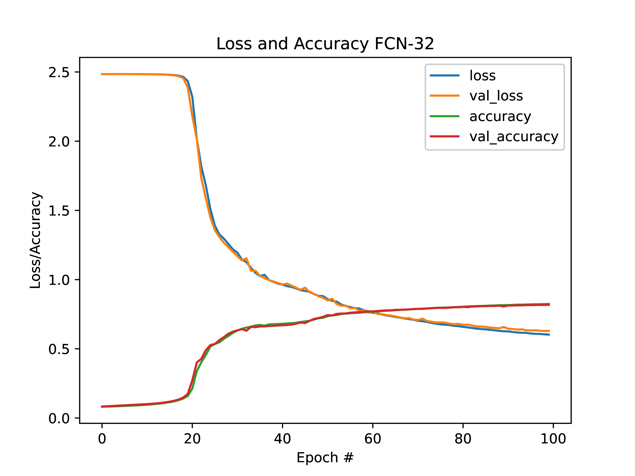
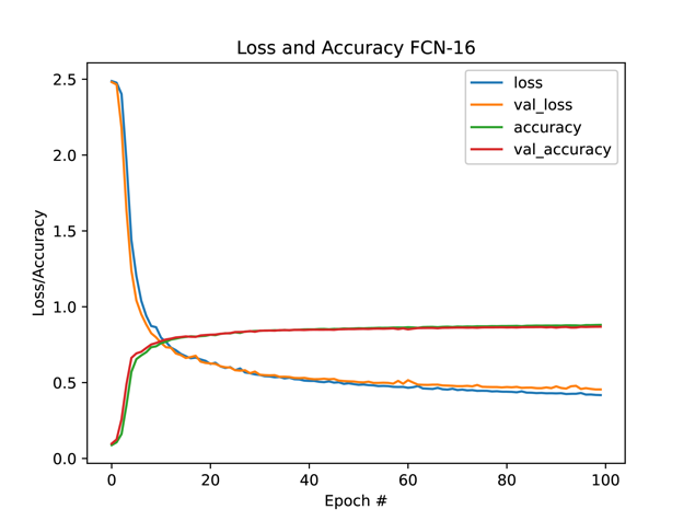
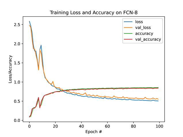
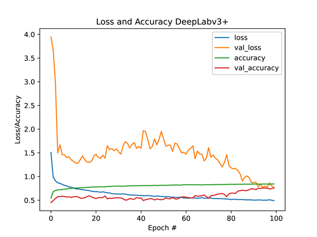
Figure 5. Loss and accuracy for different models in the first 100 epochs

To our great surprise, FCN-16 has the best performance among all four models when running for the same number of epochs, which is 100 in this case. It converges rapidly and is stable. Although we believe it will continue to converge when running more epochs, it gives a satisfying output in barely tens of epochs.

The FCN-8 model exhibits unexpected behavior around the ninth epoch, where it regresses. Subsequently, its training performance continues to fluctuate, with both loss and accuracy showing instability. This inconsistency, coupled with its lower accuracy, renders it less effective than the FCN-16 model, despite its capacity to encapsulate a broader perspective of the input.

The DeepLabv3 model, on the other hand, is a total disaster. The loss and accuracy on the training data converge stably as expected, but on the validation set, they dance across everywhere. Predicting future loss and accuracy is not easy, so early-ending conditions may be falsely triggered, leaving the model not completely trained. Even if the model converges in the last, it would take many more epochs than the FCN models.

4.3. Insights to the models

We initially anticipated that DeepLab models would outperform FCN models. However, our testing revealed otherwise, indicating that newer generations of models do not always surpass their predecessors in performance. Upon examining the theoretical underpinnings of these models, we identified several factors potentially impacting DeepLab’s performance:

• Data size limitations. DeepLab models likely require more extensive datasets to leverage their full capabilities. With smaller datasets, there may not be sufficient data for the model to stabilize its learning process, potentially leading to the fluctuations observed.

• Parameter tuning. While most parameters within the model are adjusted during the training phase, some, including learning and dilation rates, are preset within the model's architecture. Fine-tuning these parameters could enhance performance. However, there is a risk that such adjustments may only be beneficial for the specific dataset used and may not generalize well to others, reverting the model to its baseline performance.

• Model complexity. The inherent complexity of DeepLab models, compared to FCN models, might result in overfitting, particularly with smaller datasets. In such instances, a simpler model could be more effective.

These insights suggest that while DeepLab models offer advanced capabilities, their optimal application and performance are contingent upon careful consideration of dataset characteristics, parameter settings, and model complexity.

5. Conclusion

The Fully Convolutional Network (FCN) models and the DeepLab family represent effective frameworks for semantic segmentation, typically achieving high accuracy. Their performance largely depends on the availability of extensive datasets. When constrained to smaller datasets, their behavior diverges from expectations, particularly for models anticipated to excel.

Among them, the FCN-16 model emerges as the most effective, demonstrating the lowest loss and highest accuracy and Intersection over Union (IoU) metrics. Its rapid convergence rate further underscores its suitability for applications requiring real-time training. On the other hand, DeepLab models exhibit suboptimal performance on smaller datasets. To unlock their full potential, it is advisable to provide them with as much data as possible, highlighting the critical role of data volume in achieving optimal model performance.

References

[1]. George Cybenko. Approximation by superpositions of a sigmoidal function. Mathematics of control, signals and systems, 2(4):303–314, 1989.
[2]. Simon Haykin. Neural networks: a comprehensive foundation. Prentice Hall PTR, 1998.
[3]. Hamed Habibi Aghdam, Elnaz Jahani Heravi, Hamed Habibi Aghdam, and Elnaz Jahani Heravi. Convolutional neural networks, 2017.
[4]. Jonathan Long, Evan Shelhamer, and Trevor Darrell. Fully convolutional networks for semantic segmentation, 2015.
[5]. Liang-Chieh Chen, George Papandreou, Iasonas Kokkinos, Kevin Murphy, and Alan L. Yuille. Semantic image segmentation with deep convolutional nets and fully connected crfs, 2016.
[6]. George Papandreou, Iasonas Kokkinos, and Pierre-André Savalle. Untangling local and global deformations in deep convolutional networks for image classification and sliding window detection, 2014.
[7]. Liang-Chieh Chen, George Papandreou, Iasonas Kokkinos, Kevin Murphy, and Alan L. Yuille. Deeplab: Semantic image segmentation with deep convolutional nets, atrous convolution, and fully connected crfs, 2017.
[8]. Liang-Chieh Chen, George Papandreou, Florian Schroff, and Hartwig Adam. Rethinking atrous convolution for semantic image segmentation, 2017.
[9]. Liang-Chieh Chen, Yukun Zhu, George Papandreou, Florian Schroff, and Hartwig Adam. Encoder-decoder with atrous separable convolution for semantic image segmentation, 2018.
Cite this article
Yang,H. (2024). Efficiency in constraint: A comparative analysis review of FCN and DeepLab models on small-scale datasets. Applied and Computational Engineering,75,19-30.
Data availability
The datasets used and/or analyzed during the current study will be available from the authors upon reasonable request.
Disclaimer/Publisher's Note
The statements, opinions and data contained in all publications are solely those of the individual author(s) and contributor(s) and not of EWA Publishing and/or the editor(s). EWA Publishing and/or the editor(s) disclaim responsibility for any injury to people or property resulting from any ideas, methods, instructions or products referred to in the content.
About volume
Volume title: Proceedings of the 2nd International Conference on Software Engineering and Machine Learning
© 2024 by the author(s). Licensee EWA Publishing, Oxford, UK. This article is an open access article distributed under the terms and
conditions of the Creative Commons Attribution (CC BY) license. Authors who
publish this series agree to the following terms:
1. Authors retain copyright and grant the series right of first publication with the work simultaneously licensed under a Creative Commons
Attribution License that allows others to share the work with an acknowledgment of the work's authorship and initial publication in this
series.
2. Authors are able to enter into separate, additional contractual arrangements for the non-exclusive distribution of the series's published
version of the work (e.g., post it to an institutional repository or publish it in a book), with an acknowledgment of its initial
publication in this series.
3. Authors are permitted and encouraged to post their work online (e.g., in institutional repositories or on their website) prior to and
during the submission process, as it can lead to productive exchanges, as well as earlier and greater citation of published work (See
Open access policy for details).