1. Introduction

At the dawn of computers, some early games included some basic elements of artificial intelligence. However, the use of AI in games is very limited due to computational power and technical limitations. In 1950, Alan Turing published an important paper in which he proposed the concept of a chess program [1]. The publication of this paper marked the beginning of the field of AI in computer games and board games. Although computer performance was very limited at that time, it could not achieve satisfactory results in real games. The paper laid the foundation for research in this field. During that era, Arthur Samuel became the first to develop what we now recognize as reinforcement learning using a program that learned to play Checkers by playing against itself [2, 3].

The modern paradigm of chess programming began to take shape during the 1970s and early 1980s and has since undergone continuous refinement [4]. This approach relies on alpha-beta pruning [5] and the MiniMax search algorithm, further augmented by specialized extensions designed to address unique scenarios like critical forcing variations [6]. This combination of techniques has laid the foundation for developing and optimizing chess-playing AI systems. Early AI research was predominantly focused on board games. The primary rationale behind this was the inherent clarity of rules and well-defined victory conditions in these games. For instance, in chess, achieving checkmate or forming a line of five stones in games like Gomoku represent unequivocal win conditions. These characteristics simplified the formalization of problems, enabling researchers to precisely define the game states, legal moves, and victory conditions (typically expressible effectively through states and permissible actions, usually no more than approximately 100 reasonable moves available from any given position [5]).

This paper profoundly delves into classical board game AI, such as Chess and Go, focusing on their algorithms, especially AlphaGo. We will detail how these AI algorithms work. In computer science and artificial intelligence, classical board game AI research has far-reaching significance. This paper aims to provide insight for a diverse audience, from AI beginners to enthusiasts interested in board games to professionals and researchers. This is a great starting point for beginners in AI to understand the basics of the field and build a solid academic foundation by exploring well-known board game AI programs and algorithms. For those interested in board games, this paper will reveal the inner workings of these games and provide them with valuable insights for improving their game skills. Finally, for professionals and researchers alike, the study will provide the latest insights into AI algorithms and promote the application of AI technologies in a broader range of fields. By delving into classical board game AI, we can better understand how intelligent systems operate in complex decision-making environments and provide insights and inspirations for future developments in the field of AI.

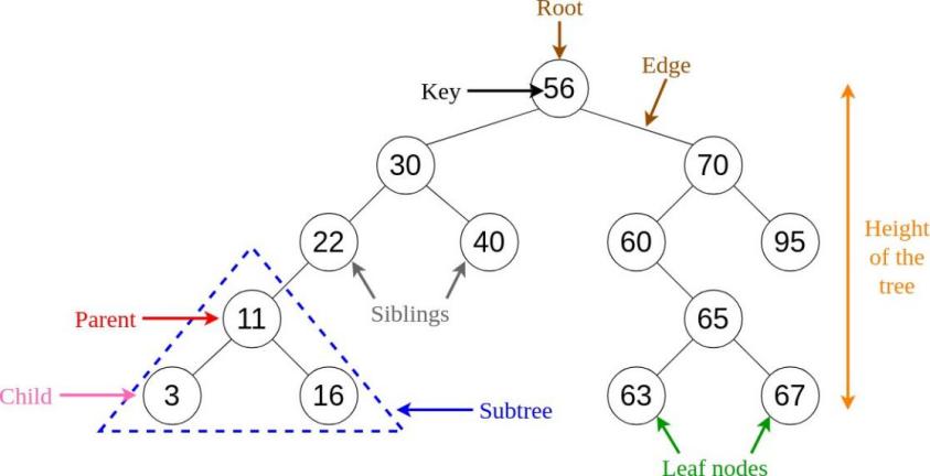
Figure 1. the whole process of MCTS

2. Algorithms in Board AI

2.1. Tree Search Algorithm

In the context of board games, the Tree Search Algorithm involves imagining the possible actions and the resulting outcomes. When taking action from a state, it leads to a new state, and this process is iterated until it reaches a final state, each corresponding to a specific value. This systematic exploration of all possible actions and consequences forms a search tree (see Figure 1). The objective is to select the action at the initial state that maximizes its associated value, where the value of a state is equivalent to the value of an action taken from it. The value of the final state, which corresponds to a leaf node, is known. To compute the values of preceding states or nodes, knowledge of the values of later states is required. This fundamental distinction from reinforcement learning lies in planning through simulated scenarios instead of learning from real experiences. In the Tree Search Algorithm, several critical components are involved. A node is a fundamental unit, with the foremost node referred to as the root. Leaf nodes represent the endpoints of the tree, and actions connecting nodes are known as edges. Nodes are interconnected through edges, forming parent-child relationships between them. For example, the root node is the parent of every node in the layer below, and each leaf node is a child of the corresponding node in the layer above.

When two players, the agent and the rival, are engaged, the agent's actions begin with the current state as the root. The search expands by imagining all possible actions (outcomes) at the first level, leading to the creation of edges (agent actions) and nodes (outcomes). From the agent's perspective, the rival's actions are treated as states, while the agent's possible actions are outcomes. The process continues by considering the rival's potential actions and consequences, followed by the agent's actions and outcomes. Once this process stops, the final layer of nodes constitutes the leaf nodes, marking the completion of the search tree. Subsequently, the values of these leaf nodes are calculated, typically through manually defined functions that consider various board features, such as the quantity and types of game pieces. These values, known as naive values, are then propagated through the tree's nodes and edges, referred to as backup. Ultimately, the values of actions and edges at the initial level are determined, enabling the selecting of the action with the highest value.

2.2. MiniMax Tree Finding

The MiniMax algorithm is a backup operation for calculating node values in a game tree. Assuming we have already obtained the values of leaf nodes, the next step is to compute the values of higher-level nodes. At this node level, the agent needs to choose an action. The agent will select the action with the maximum value, so the value of this node equals the maximum value among its child nodes. Similarly, we can calculate the values of other nodes at the same level by passing the values of leaf nodes up to the parent nodes. We then continue this propagation upwards. In the parent nodes at the upper level, the rival needs to select an action, and thus, the rival will choose the action that leads to the minimum value. This is because the value is relative to the agent, and the agent prefers higher values as they are more advantageous. Therefore, the value of this node equals the minimum value among its child nodes. In the MiniMax algorithm, the value of agent nodes is determined by choosing the maximum value among their child nodes. In contrast, the value of rival nodes is determined by selecting the minimum value among their child nodes. Hence, this algorithm is known as MiniMax.

In 1997, the Deep Blue computer [7], which defeated the world chess champion, employed the MiniMax tree search algorithm. However, the MiniMax algorithm faces a problem wherein the search tree grows exponentially, as each node considers all possible actions and their consequences, and each consequence leads to multiple possible actions. To address this issue, Deep Blue also utilized a technique to reduce the size of the search tree, known as Alpha-Beta pruning. Additionally, the MiniMax algorithm typically limits the number of levels it searches rather than exploring all the way to the deepest level.

2.3. Alpha-beta Pruning

In the process of constructing the search tree, we don’t obtain all leaf nodes simultaneously; instead, we acquire them one at a time. We can perform a backup operation when we have obtained all the values of a parent node’s leaf nodes (child nodes). After obtaining the value of the first node in the second-to-last layer, we continue exploration and calculate the value of the first child node of the second node. It is important to note that the value of the second node must be greater than or equal to the value of its first leaf node (since we always select the maximum value regardless of the other leaf node’s value). We choose the minimum value when we reach the third-to-last layer, which corresponds to the rival’s actions. If the value of its first child node is smaller than the range of values for the second child node, it is unnecessary to explore that particular node. We then proceed to explore the parent nodes of other leaf nodes. By using the value of these parent nodes, we can deduce that the corresponding nodes at the upper layer (rival state) can have a value at most equal to the parent node’s value. When comparing the values of nodes at the same parent node for the rival state, the agent state will choose the maximum value. Consequently, some child nodes can be explored without exploring. This process continues, and some remaining leaf nodes can be left unexplored. Through this algorithm, we effectively reduce the size of the search tree, thereby improving search efficiency.

Ultimately, we obtain the first-layer edges, and the agent selects the action with the highest value as its actual move. This leads us to a real rival state. The rival also makes a real move based on its considerations, entering a real agent state. This state becomes a new root node, initiating the MiniMax research process anew. Consequently, in Deep Blue’s chess gameplay, each move is determined through the search tree, in contrast to reinforcement learning, where a policy function decides actions. However, it is worth noting that this policy function can also be employed in the tree search process.

2.4. Monte Carlo Rollout

Monte Carlo Rollout is a game tree search technique designed to evaluate the value of the current game state. It works by estimating a state's value through simulating the game's progression, as opposed to fully expanding the entire game tree, which is typical in MiniMax algorithms. To begin with, starting from the current game state, we consider all possible actions and their corresponding consequences, forming the first layer of edges and nodes. This layer consists of the last layer of nodes and leaf nodes, resulting in a relatively shallow game tree. Next, we initiate the Rollout process starting from each leaf node. In Rollout, we randomly select an action and simulate the game's progression until it reaches an end state. This Rollout process is repeated multiple times (typically controlled by an adjustable hyperparameter, n) to generate winning probabilities for each leaf node. These winning probabilities are then used as the values of the leaf nodes.

Subsequently, the agent makes its actual move based on these leaf node values, selecting the action with the highest value. Following this, we enter a new root node and continue the Monte Carlo Rollout to improve the estimation of state values iteratively. It is important to note that as the number of Rollout iterations (n) increases, the Rollout values gradually converge to approximate the true state values.

Unlike the traditional MiniMax algorithm that considers the entire game tree, Monte Carlo Rollout only focuses on the first layer of nodes, with subsequent iterations involving single action selections. The Rollout policy determines the specific action choices. This approach offers the advantage of providing valuable value estimates in scenarios with a large state space or when precise modeling is challenging. Therefore, Monte Carlo Rollout finds extensive applications in games and decision-making problems.

2.5. Monte Carlo Tree Search (MCTS)

Monte Carlo Tree Search (MCTS) is a powerful game tree search algorithm that combines Monte Carlo Rollout and MiniMax tree search elements. It is particularly effective in scenarios where the game tree is too large for exhaustive exploration.

The MCTS algorithm starts from a common root node. Initially, it employs the MiniMax tree search technique to build a relatively deep but not fully expanded search tree. Then, it proceeds with Monte Carlo Rollout, starting from the leaf nodes, and repeats this process for a specified number of iterations (denoted as \( N \) ). A tree policy is used throughout the tree search process to guide the exploration. During the Rollout phase, the algorithm estimates the value of each leaf node by conducting Monte Carlo simulations. These estimated values are referred to as the “Rollout values” and serve as the leaf nodes’ values. Subsequently, the algorithm integrates the Rollout values into the search tree using the principles of MiniMax tree search. It propagates the leaf nodes’ values upwards in the search tree. After conducting a certain number of iterations, MCTS selects the action with the highest value as the actual move. By combining these two methods, MCTS aims to enhance the accuracy of value estimation. However, it is worth noting that the computational complexity of both techniques combined does not always lead to a substantial improvement in performance.

The core iteration of the general MCTS approach involves the following steps, as illustrated in the figure 2 below.

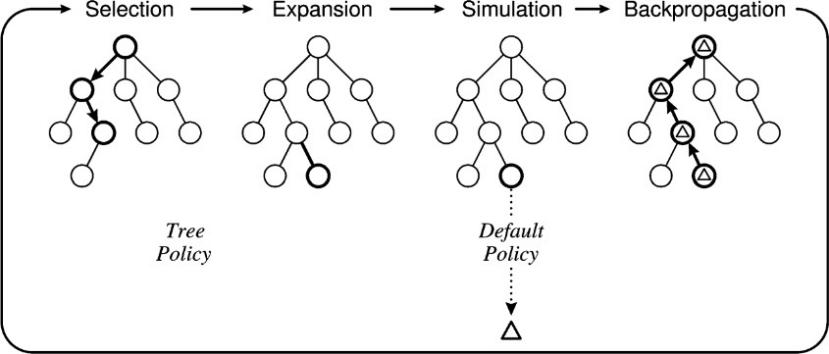
Figure 2. the whole process of MCTS

In the initial stage, each edge in the first layer is associated with two variables: \( Q(s, a) \) and \( N (s, a) \) , where s represents the state, and \( a \) represents the action. The variable \( Q(s, a) \) denotes the average or positional value of choosing action a in state s, while \( N (s, a) \) represents the frequency or count of choosing action a in state s. Both \( Q \) and \( N \) are initialized to 0. MCTS operates iteratively, expanding the search tree, conducting Rollouts, and updating the Q and N values until a stopping criterion is met. This dynamic and adaptive approach makes MCTS a versatile algorithm for various games and decision-making problems.

2.5.1. Selection

In the Monte Carlo Tree Search (MCTS) algorithm, the next step is to employ a tree policy known as UCT (Upper Confidence Bounds for Trees) to choose the node for exploration.

According to the UCT policy, we first consider all possible actions that can be taken from the current node, along with their consequences, forming the first layer of edges and nodes. The nodes in this layer are essentially the leaf nodes. However, since all actions in the first layer are equivalent, we typically choose one action at random based on a certain probability, rather than selecting a specific node. This process is referred to as” selection.”

When selecting an action, we use the following UCT formula (Equation 1) [8]:

\( A=arg{\underset{a∈A(s)}{max}}\lbrace Q(s,a)+C\sqrt[]{\frac{ln{[N(s)]}}{N(s,a)}}\rbrace \) (1)

In this formula, \( Q(s, a) \) represents the average return or value of a node, \( N (s, a) \) represents the number of times the node has been visited, and \( C \) is an exploration parameter that controls the weight of exploration. The first part of the formula \( Q(s, a) \) represents the average value, which is higher for actions that lead to a higher average return, making them more likely to be chosen. The second part of the formula \( C\sqrt[]{\frac{ln{[N(s)]}}{N(s,a)}} \) represents uncertainty, and by increasing the exploration parameter \( C, \) we can increase the weight of exploration, favoring the selection of less explored actions to balance the trade-off between exploration and exploitation. This means that actions with fewer visits are more likely to be chosen.

It’s important to note that during the selection phase, we typically choose only one action from all actions in the first layer, rather than selecting all actions at once. This process is guided by the policy function and involves selecting one action based on certain probabilities. After selecting an action, the corresponding edge’s visit count is updated to 1, and other actions are temporarily ignored.

2.5.2. Simulation and Backup

Next, starting from the chosen leaf node, we perform a “rollout” in which we simulate a game until it reaches its conclusion. In each simulation, the result, whether a win or loss, is recorded as the value (typically 1 for a win and -1 for a loss) returned to the leaf node. We then calculate the total value of the leaf node, often denoted as \( W (s, a) \) , where \( W(s,a)=\sum V({s_{leaf}}) \) , and \( V ({s_{leaf}}) \) represents the win/loss results of each simulation.

Subsequently, we compute the \( Q \) value for the edge:

\( Q(s, a)=\frac{W (s, a)}{N (s, a)} \) (2)

where the \( Q \) value represents the average value of all leaf nodes associated with the action. This average value becomes the value associated with the action itself.

This computational process is referred to as “backup” because we are propagating the results of simulations back into the search tree. We then return to the “selection” phase, starting the selection process again using the UCT policy. During the new selection process, the visit count of the corresponding edge is updated to 1, and simulations start anew, yielding new results that are propagated back in the same manner.

2.5.3. Expansion and Backup

MCTS includes an optional step called “expansion”. Expansion involves transforming a leaf node into an internal node and continuing exploration within that internal node. Without expansion, a leaf node will be iteratively used multiple times, gradually increasing its visit count. When the visit count reaches a certain threshold (typically used for dynamic adjustment to control the growth rate of the search tree), the expansion step is triggered.

The leaf node is transformed into an internal node during the expansion process. Then, possible actions and resulting states from the new internal node are considered, forming new edges and nodes with new \( Q \) and \( N \) values. Simulations are then conducted within the new leaf nodes. The results of these new simulations are also propagated back into the search tree, updating the relevant \( Q \) and values.

The purpose of expansion is to make the search tree more dynamic, enabling a more comprehensive exploration of the state space. It is important to note that some leaf nodes may be chosen during expansion, while others may not, depending on the selection strategy based on the UCT policy.

2.5.4. Conclusion

In conclusion, Monte Carlo Tree Search (MCTS) constructs a search tree through a continuous process of “selection,” “simulation,” and “backup.” Each edge in the search tree corresponds to a state-action pair and maintains three variables: \( Q(s, a) \) , \( N (s, a) \) , and \( W (s, a) \) .

The ultimate goal is to select an action from the first layer of edges in the search tree. Typically, we choose the action with the highest visit count \( N \) , as this selection criterion is relatively stable in practice and less affected by extreme values. After the agent selects an action, the opponent (rival) also chooses an action, and the process enters the next agent’s state, initiating a new round of MCTS search. In this process, the results of the previous round’s search tree can be inherited and used in the new round.

Overall, MCTS combines the strengths of MiniMax tree search and Monte Carlo simulation algorithms, while efficiently utilizing value and policy functions to make tree search highly effective.

2.6. MCTS with Deep Neural Networks: AlphaGo

AlphaGo leverages the synergy between Monte Carlo Tree Search (MCTS) and deep neural networks to significantly enhance its performance in the game of Go. This fusion capitalizes on the crucial role played by deep neural networks, leading to a substantial improvement in the efficiency of the Monte Carlo search. Simultaneously, MCTS’s forward-looking search capability helps compensate for the limitation of policy networks, which rely solely on the current state of the game board. AlphaGo employs a search algorithm that combines Monte Carlo simulation with two neural networks: a value network and a policy network. The policy network further subdivides into the rollout policy network, supervised learning policy network, and reinforcement learning policy network.

In AlphaGo, DeepMind constructs the game board positions using convolutional neural networks (CNN) and extensively utilizes neural networks to enhance the efficiency and accuracy of the search tree [9]. Specifically, the value network is responsible for assessing the value of each game board position, while the policy network is tasked with selecting the next move. The roles of these two deep neural networks in the MCTS process can be categorized into the following stages: selection (tree policy), simulation (rollout policy), and Backup.

AlphaGo employs supervised learning to train two policy networks, which guide the selection of AlphaGo’s next moves. The supervised learning policy networks take the current game board state as input and output probabilities for different actions after processing through the neural network. Additionally, AlphaGo employs reinforcement learning to train two deep neural networks, namely, the policy network and the value network. The objective of reinforcement learning is to secure victories in actual games, rather than merely replicating expert gameplay. Consequently, the policy network and the value network undergo continuous self-play and strategy optimization, ultimately achieving remarkable performance.

2.6.1. Supervised Learning Policy Network

In the field of artificial intelligence for Go, the Supervised Learning Policy Network plays a pivotal role. Its primary objective is to enhance autonomous decision-making by emulating the choices of human Go players. This network, implemented as a deep convolutional neural network (CNN), takes the current state of the board as input and outputs a probability distribution over the empty spaces on the board where a professional Go player would make their next move. DeepMind conducted training for a policy network using a dataset comprising 30 million positions from the KGS Go Server, achieving remarkable results with an accuracy of 57 percent in just 3 milliseconds [9].

The training process of the SL policy network includes the following key steps: first, a substantial amount of training data is collected, with each board state being fed into the network. The network then performs forward propagation and computes the loss function to measure the disparity between the network’s output and the correct moves of professional players. Subsequently, optimization algorithms such as gradient descent are utilized to iteratively adjust the network’s weights and biases to minimize the loss function. This process is iterated repeatedly, with each iteration providing more game records that gradually enhance the network’s performance through gradient descent updates. The ultimate goal of the entire training process is to enable the SL policy network to predict Go moves similar to those of professional players in any given board state. Once the training is complete, this SL policy network can guide AlphaGo in selecting optimal moves during the search process, significantly improving the efficiency and quality of the search. Whenever a board position is input, the network returns a probability distribution over potential move.

2.6.2. Rollout Policy Network

The Rollout Policy Network, also known as the Fast Rollout Policy Network, plays a critical role in Monte Carlo Tree Search (MCTS). MCTS employs the Rollout Policy Network to perform a series of random simulations to evaluate the effectiveness of taking different actions in the current game state. In normal simulations, Rollouts often require hundreds of steps to determine the game's final outcome, making it computationally intensive. Therefore, there is a need for a policy function that can make quick selections, achieved through training a simple neural network as the Rollout policy.

The training objective of the Rollout policy network is similar to that of the Supervised Learning (SL) policy network—both aim to emulate expert action selection to improve decision-making during the Monte Carlo Tree Search. DeepMind used 8 million human expert state-action pairs to train this network [9]. Ultimately, it can complete calculations in just 2 microseconds, which is one-thousandth of the time required by the SL network, but its accuracy is only 24.2 percent [9]. Similar to the SL policy network, data collection for the Rollout policy network is based on game records of professional players, including board states and corresponding correct actions. However, the rollout policy network differs in that it linearly combines attributes of each board state (such as board position, average value, visit count, etc.) to generate a vector representing the board state.

This step aims to transform the current state of the board into a numerical vector that the neural network can process. This vector serves as the input to the Rollout Policy Network, which then outputs a probability distribution over all possible actions. Since this is a probability distribution, the Softmax function is typically used to convert it into probability values. During training, the network adjusts its weights to minimize the loss function, bringing its output probability distribution closer to the correct action distribution. This constitutes the entire training process, and through multiple rounds of training, the network's output becomes more accurate, resembling human action choices.

Once training is complete, the Softmax function generates probabilities for each possible action whenever the current board state is input. Thus, in AlphaGo's MCTS, the Rollout process involves linearly combining the current board state, using weights to weigh different features to generate a vector representing the current game situation. Subsequently, the Softmax activation function yields a probability distribution for each possible action. Finally, based on the probability distribution output by Softmax, the Rollout Policy selects the following action. In other words, the Rollout Policy's process first selects a leaf node for expansion in the selection part, then inputs the current situation into the Rollout Policy Network to perform a series of random simulations (rollouts). In each simulation, we obtain probabilities for each action in the current situation and then use a certain strategy to select the next action (usually the action with the highest probability for movement). This process is repeated until a terminal state is reached (e.g., the game result is determined). This constitutes the entire simulation process.

What sets the trained Rollout Policy apart from a traditional rollout is that the Rollout Policy Network is trained through supervised learning, guided by expert data, and employs deep reinforcement learning techniques for more precise action evaluation and selection. Its strategy is closer to that of human experts rather than being entirely random. Traditional random rollouts typically estimate action values through multiple random simulations without using deep reinforcement learning. However, unlike the Supervised Learning policy, this network sacrifices the quality of moves to achieve faster move generation.

Unlike the SL policy, the Rollout policy extracts local features and trains a linear model based on them. In contrast, the SL policy network utilizes global features and deep learning models for training.

2.6.3. Reinforcement Learning Policy Network

The Reinforcement Learning (RL) policy network is also a deep convolutional neural network. The RL policy network is initialized with the Supervised Learning (SL) policy network, and it is continuously optimized through self-play while adjusting the optimization objectives based on the original supervised learning network. Its primary focus is not only to mimic expert moves but to win games.

In the RL training process, the previously trained policy network plays against a randomly selected previous version of itself. The Policy Gradient Algorithm is then employed to train the RL policy network. If an action leads to a higher reward (winning), its probability of occurrence is increased, and if an action leads to a lower reward (losing), its probability is decreased. The primary principle is to maximize rewards to adjust the probabilities of actions. This entire process involves reinforcement learning. After training, the RL policy network achieves a win rate of approximately 80 percent when playing against the supervised learning network [9].

2.6.4. Value Network

The Value Network in reinforcement learning is a neural network used to evaluate the value of a game state. Its primary task is to estimate how likely AlphaGo is to win or lose in the current game state. It is trained using regression with the objective of minimizing mean squared error through stochastic gradient descent. The training method for the Value Network also involves reinforcement learning. It uses policy gradient methods to continually improve the performance of the reinforcement learning value network. Through iterative processes and parameter updates, the goal is to enhance the estimation of win rates in game states.

During the self-play process of the RL policy network in reinforcement learning, a new dataset is generated. To prevent overfitting, the training data for the Value Network is derived from 30 million board positions generated by self-play from the trained RL policy network. Each board position is sampled from individual complete games. However, the training data is collected diversely during each game. This includes using the SL policy network to make moves for the first n moves, followed by random moves, and finally relying on the RL policy network to make moves until the game’s conclusion. This diverse data collection approach helps increase the diversity of training data to guard against overfitting.

In summary, the purpose of the Value Network is to use it to evaluate the likelihood of winning a game state. This deep network is used in conjunction with the Rollout Policy Network during the simulation process to determine the value of leaf nodes.

2.6.5. Process of MCTS in AlphaGo

In AlphaGo, the Monte Carlo Tree Search (MCTS) process involves several crucial steps. Firstly, it is imperative to train the policy model, rollout model, and value model offline. Then, the MCTS process follows the conventional flow, starting from the root node and progressively generating edges for each layer and nodes for the first layer. The unique aspect here is the integration of the supervised policy network into the tree policy. The approach adopted is PUCT (Probabilistic UCT), which essentially combines UCT with an SL policy. At each time step t during a simulation, an action a is selected from states using the formula:

\( A=argmax\lbrace Q(s, a)+ u(s, a)\rbrace \)

\( a∈A(s) \) (3)

Here, \( Q \) represents the average value, and \( u(s, a) \) is a bonus term, computed as:

\( u(s, a)∝\frac{P (s, a)}{1+N(s,a)} \) (4)

The numerator represents the probability of action an obtained from the supervised policy network, while the denominator accumulates the count of selecting that action in simulations up to the current step. This bonus term ensures that the average value is directly proportional to the action’s prior probability \( P (s, a) \) and inversely proportional to the number of times \( N (s, a) \) the action has been chosen. Consequently, PUCT tends to explore paths with high prior probabilities P and low visit counts, which haven’t been extensively explored. From another perspective, due to this supervised learning strategy, the focus can be on actions with high probabilities from the outset, eliminating the need for a gradual learning curve as in the traditional UCT. This considerably enhances the efficiency of MCTS tree search.

It’s worth noting that although reinforcement learning networks are more potent, AlphaGo employs an SL policy rather than an RL policy for PUCT. In practical terms, SL POLICY results are better suited for MCTS searches. While both policies serve the same purpose of providing a prior bias for action selection, SL policy, being closer to human choices, offers a broader range of action choices. Human choices involve a diverse spectrum of promising moves, thereby widening the selection range. Conversely, after further optimization, RL policy narrows down the selection range. When training the value network, the objective is to determine the final win rate if both sides play optimally. This is why the strongest RL policy is utilized for training.

Using this strategy, we select an action, enter a new leaf node as in the previous step, and then start rollout, or simulation. Here, we no longer employ a random strategy but rather utilize a learned rollout policy. This policy is chosen for its computational efficiency, enabling us to swiftly simulate an entire game and obtain a result. Ultimately, we obtain a rollout result denoted as r (+1 for winning and -1 for losing).

Next comes the backup step, where, in MCTS, we assign the result obtained from the rollout as the value to the leaf node. However, in AlphaGo, the evaluation of a leaf node occurs in two ways: one is the win rate \( {V_{0}} \) of that leaf node derived from the value network, and the other is a rollout value r obtained from the rollout policy. We pass the rollout result \( r \) to the leaf node and calculate the value V for the leaf node through a weighted average. The equation for calculating \( V \) is as follows:

\( V (s) = (1 - λ) × V0(s) + λ × z \) (5)

Here, \( V (s) \) represents the value of the leaf node, \( {V_{0}} \) is the win rate obtained for the leaf node through the value network, and r represents the rollout value. The remaining steps are similar to MCTS: we calculate and update the total value W and the average value Q for the leaf node and all its ancestors, along with updating the visit count \( N \) . We may also adjust parameters and weights for functions like PUCT.

In conclusion, one iteration of Monte Carlo tree search in AlphaGo consists of the following steps: 1. Extracting relevant features based on the current state of the board and the moves made so far. 2. Estimating the probabilities P of placing stones in unoccupied positions on the board using the SL learning policy network. 3. Inputting the placement probabilities P into the PUCT function to obtain the A and determining the next node to visit by selecting the action with the highest \( A . \) 4. Expanding a node if the visit count of a leaf node reaches a predefined threshold. 5. After selecting the leaf node for simulation, assessing the game’s value separately using the value network and rollout policy network, and then calculating the leaf node’s temporary value V through a weighted average. 6. Backing up the values through the transmission of information and updating the attributes of nodes.

3. AI from DeepMind

3.1. Alphago

On March 9, 2016, AlphaGo achieved a monumental victory against the seventeen-time world Go champion, Lee Sedol, with a score of four to one. Behind this remarkable feat lay the utilization of two neural networks: one being the policy network, employed to narrow the search space by retaining high-probability nodes and discarding low-winning probability moves; the other being the value network, used to assess the board’s positional value. Despite AlphaGo reaching the pinnacle of human performance at that moment, it did not entirely dominate humanity. In the fourth game of the man-versus-machine showdown, Lee Sedol secured a miraculous victory with his” Divine Move,” demonstrating the ingenuity of the human mind. However, nine months later, AlphaGo Master [10] emerged onto the stage, achieving a flawless 60: 0 record against numerous world-class Go players, including Ke Jie. Following this, the Go world embarked on a new era, a revolutionary era – the era of AlphaGo Zero [10].

3.2. Alphago Zero

AlphaGo Zero [10] has achieved remarkable feats, surpassing human performance with an astonish- ing record of 100 wins to 0 losses, even surpassing the previous version of AlphaGo that defeated Lee Sedol.

AlphaGo Zero stands apart from its predecessors in several significant ways. Firstly, it relies entirely on self-play and reinforcement learning, devoid of any dependence on human expertise or knowledge. Given the fundamental rules of Go, AlphaGo Zero gradually elevates its own capabilities through self-play and training. Unlike previous versions, AlphaGo Zero utilizes a single neural network, eliminating the need for separate policy and value networks. Additionally, it employs an entirely new reinforcement learning algorithm, diverging from traditional Monte Carlo Tree Search distributions. What’s truly astonishing is that AlphaGo Zero, in a mere 40 days, achieved its current high level of performance through approximately 29 million games of self-play training [10].

3.3. Alphazero

Alpha Zero [11] is, in fact, a derivative of AlphaGo Zero, and its overall framework and principles closely resemble those of the original AlphaGo Zero. However, it introduces further refinements to the existing algorithm to master chess and shogi, among other games.

AlphaZero still relies on key components such as deep neural networks and Monte Carlo Tree Search (MCTS). However, it utilizes a distinct training dataset tailored to its need to learn various board games with different rules. This broadens its applicability to a wider range of games.

4. Conclusion

In conclusion, the advancements in AI showcased through board games like Go have reshaped the landscape of artificial intelligence. The journey from Alphago’s historic victory to the remarkable feats of AlphaGo Zero and Alpha Zero demonstrates the power of deep neural networks and reinforcement learning in conquering complex challenges. These achievements not only signify AI’s prowess in mastering strategic games but also serve as a catalyst for innovation in diverse domains.

References

[1]. Turing, A. M. Digital computers applied to games. Faster than thought (1953).
[2]. Garc´ıa-S´anchez, P. Georgios n. yannakakis and julian togelius: Artificial intelligence and games: Springer, 2018, print isbn: 978-3-319-63518-7, online isbn: 978-3-319-63519-4, https://doi. org/10.1007/978-3-319-63519-4. Genetic Programming and Evolvable Machines 20, 143–145 (2019).
[3]. Samuel, A. L. Some studies in machine learning using the game of checkers. ii—recent progress. IBM Journal of research and development 11, 601–617 (1967).
[4]. Slate, D. J. & Atkin, L. R. Chess 4.5—the northwestern university chess program. Chess skill in Man and Machine 82–118 (1977).
[5]. Risi, S. & Preuss, M. From chess and atari to starcraft and beyond: How game ai is driving the world of ai. KI-Ku¨nstliche Intelligenz 34, 7–17 (2020).
[6]. Levinson, R., Hsu, F.-H., Marsland, T. A., Schaeffer, J. & Wilkins, D. E. Panel: The role of chess in artificial intelligence research. In Proceedings of the 12th International Joint Confer- ence on Artificial Intelligence (1991).
[7]. Campbell, M., Hoane Jr, A. J. & Hsu, F.-h. Deep blue. Artificial intelligence 134, 57–83 (2002).
[8]. S´wiechowski, M., Man´dziuk, J. & Ong, Y. S. Specialization of a uct-based general game playing program to single-player games. IEEE Transactions on Computational Intelligence and AI in Games 8, 218–228 (2015).
[9]. Silver, D. et al. Mastering the game of go with deep neural networks and tree search. nature 529, 484–489 (2016).
[10]. Silver, D. et al. Mastering the game of go without human knowledge. nature 550, 354–359 (2017).
[11]. Silver, D. et al. A general reinforcement learning algorithm that masters chess, shogi, and go through self-play. Science 362, 1140–1144 (2018).
Cite this article
Liu,A. (2024). AI techniques in board game: A survey. Applied and Computational Engineering,79,49-59.
Data availability
The datasets used and/or analyzed during the current study will be available from the authors upon reasonable request.
Disclaimer/Publisher's Note
The statements, opinions and data contained in all publications are solely those of the individual author(s) and contributor(s) and not of EWA Publishing and/or the editor(s). EWA Publishing and/or the editor(s) disclaim responsibility for any injury to people or property resulting from any ideas, methods, instructions or products referred to in the content.
About volume
Volume title: Proceedings of the 4th International Conference on Signal Processing and Machine Learning
© 2024 by the author(s). Licensee EWA Publishing, Oxford, UK. This article is an open access article distributed under the terms and
conditions of the Creative Commons Attribution (CC BY) license. Authors who
publish this series agree to the following terms:
1. Authors retain copyright and grant the series right of first publication with the work simultaneously licensed under a Creative Commons
Attribution License that allows others to share the work with an acknowledgment of the work's authorship and initial publication in this
series.
2. Authors are able to enter into separate, additional contractual arrangements for the non-exclusive distribution of the series's published
version of the work (e.g., post it to an institutional repository or publish it in a book), with an acknowledgment of its initial
publication in this series.
3. Authors are permitted and encouraged to post their work online (e.g., in institutional repositories or on their website) prior to and
during the submission process, as it can lead to productive exchanges, as well as earlier and greater citation of published work (See
Open access policy for details).