1. Introduction

With the development of human society, humans continue to develop machines to adapt the needs of human life, including computing, social services, etc. The development of machines has made people's lives easier, and machine learning is one of them. Machine learning is scientific research that utilizes algorithms to accomplish specific tasks. Many services used in the daily lives are based on machine learning. For example, when people shop online, machine learning will provide them with frequently searched products, making shopping more convenient. In addition, when people use input methods, machine learning learns from databases to provide them with the text they want to type next. It can be seen that machine learning has greatly facilitated people's lives. Meanwhile, machine learning can solve some problems that traditional learning methods cannot accomplish and is a powerful tool [1, 2].

Contemporarily, with the continuous development of machine learning. The application scope of machine learning is expanding, with extensive applications in fields such as physics, medicine, and economics. Machine learning plays a relatively important role in clinical medicine, and the application of digital technology can better understand the pathology of diseases and solve problems [3, 4]. In drug development, machine learning can analyze specific problems through its own data and generate accurate predictions and insights [4]. Meanwhile, through machine learning, people can also predict diseases such as glaucoma [5]. In today's medical field, it is also necessary to promote the development of medical technology through the development of machine learning to better identify important features of diseases [4, 6].

In the field of physics, machine learning also has many applications. For example, machine learning can provide algorithms and excellent tools in multiple fields such as particle physics, cosmology, and materials science. Nowadays, the development of machine learning is also focused on researching and developing new architectures to accelerate machine learning [7, 8]. The success and development of some fields are closely related to the current development of machine learning. In the field of economics, machine learning has a certain correlation with economics and econometrics [9]. The results of machine learning often perform better than traditional methods, including government policies or consumer behavior and levels [9]. Optimization problems are also a very important part of machine learning. The complexity of data and the increase in data volume pose significant challenges to optimizing machine learning [10]. On this issue, people have been constantly developing machine learning and also challenging some emerging problems. The rapid growth of data around the world has made it increasingly difficult to extract effective data. Machine learning has also played an important role in big data processing [11, 12]. It extracts and analyzes valuable information from big data to make predictions and decisions. Overall, machine learning is increasingly being applied in the lives and plays a very important role in human development. Human beings have also been in a continuous process of developing machine learning. The different ways in which models process data affect the performance of this model. Meanwhile, the hyperparameters set by this model also deeply affect the performance of the model. This article will use learning rate as a representative hyperparameter to analyze the impact of learning rate on the convergence of the loss function through experiments, and explore the influence of learning rate on the quality of the model. In subsequent articles, the Sec. 2 will introduce the dataset MNIST used in this experiment, as well as the three models used in this experiment, namely transformer, diffusion, and RNN. In Sec. 3, the performance of these three models will be explained, and the results will be explained. This study will also explain the limitations of the experiment and provide future prospects. A summary will be provided in Sec. 4.

2. Data and method

The data used in this experiment is from a dataset called MNIST. MNIST in this experiment was found from the Dataset library in Python. MNIST is a large manual numerical dataset and the labels in the MNIST dataset are numbers ranging from zero to nine. MNIST includes 60000 training samples and 10000 testing samples. It contains many ways of writing from 0 to 9. This dataset is very common in machine learning and people often use models to train it to measure the accuracy of the models. In this experiment, it uses this dataset to discover the convergence of the loss function under different hyperparameters. In order to have a better understanding of MNIST, the following figure randomly generated twenty-five data from this dataset. One can see that the label displays numbers, and the corresponding image below is its writing form, which corresponds one-to-one. As shown in Fig. 1.

The three models of transformer, diffusion, and RNN will be applied in the experiment. Then, one will briefly introduce three models. Transformer model is a deep learning architecture that introduces self-attention mechanisms to balance the importance of different positions in the input sequence, thereby better handling long-distance dependencies. It is an important component of modern NLP research and applications. Diffusion model is a generative model based on a probabilistic diffusion process, which can generate data similar to the training set. It utilizes the inverse process of the diffusion process by learning to recover data through reversing noise. Finally, it generates data by learning the denoising process. RNN is a special type of large model neural network that introduces loops in hidden layers to enable the network to remember previous information and process the current input in datasets with dependencies. The three models train the data differently, and their best hyperparameters are different. Therefore, one only selects parameters within a certain range for experiment and comparison.

This experiment will use these three models to train MNIST and plot the loss function graph. Computer will use different models to let the machine learn these 60000 different ways of writing, and then use 10000 data points to test whether the machine can distinguish the numbers corresponding to these data. In this process, the learning rate will be used as a variable, ranging from 0.0001 to 0.001, with a change of 0.0001 each time, while other hyperparameters will remain constant. Computer will plot different loss function images with different learning rates and analyze the changes in the images. For the variation of the loss function, one will compare ten images and analyze the initial values, convergence speed, and final convergence value. The loss function is used to evaluate the degree to which the true value differs from the predicted value. Curves with faster convergence rates and smaller final convergence values are considered to have better loss functions and better demonstrate that this is a model with better performance. This is because the smaller the value of the loss function, the higher the accuracy of the test, indicating that the model has a good training effect. After analysis, the experiment will give a relatively reasonable learning rate (0.0001 to 0.001) for the three models. This study will also briefly analyze why this learning rate is the best for the model, and analyze why the optimal learning rate is different for different models from the way the model is trained.

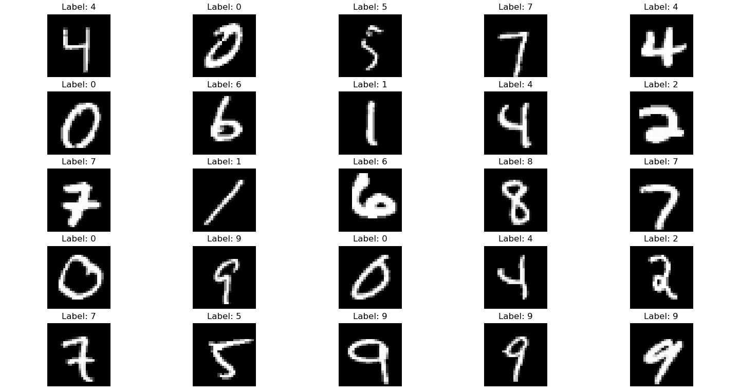
Figure 1. Labelling of the data (Photo/Picture credit: Original).

3. Results and discussion

3.1. Model performance

The first one used is the transformer model. By changing the learning rate, computer plotted ten loss function images using the transformer model. Analyze by observing three results shown in Fig. 2 with learning rates of 0.0001, 0.0002, and 0.001. These three images will be displayed below. This article will first analyze these three images, and then compare and discuss them. Firstly, when the learning rate is equal to 0.0001, one finds that the initial value is between 0.3 and 0.35. During the convergence process, the image is relatively smooth and the convergence speed is relatively fast. When epoch equals 60, the image has almost converged to 0. The final convergence result has also tended towards 0, so this is a relatively good convergence model. A learning rate of 0.0001 is also a good learning rate. Look at the image with a learning rate equal to 0.0002. Its initial value is around 0.3, and the overall convergence is also relatively fast. However, during the convergence process, fluctuations often occur, and the function does not appear very smooth. It also tends towards a convergence value of 0 when epoch equals 0. The last image shows a learning rate of 0.001, with an initial value exceeding 0.5. Its speed is relatively slow, and its convergence value with an epoch of 100 is around 0.02. This indicates that the performance of the convergence model is not very effective, and the parameter with a learning rate of 0.001 is not satisfactory. Next, this essay will compare these three graphs and find that the model performance of the first two graphs is significantly better than that of the third graph. That is to say, when the learning rate is controlled between 0.0001 and 0.001, models with a learning rate close to 0.0001 will perform better, resulting in better function convergence.

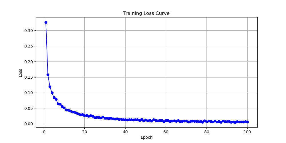
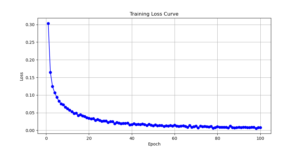
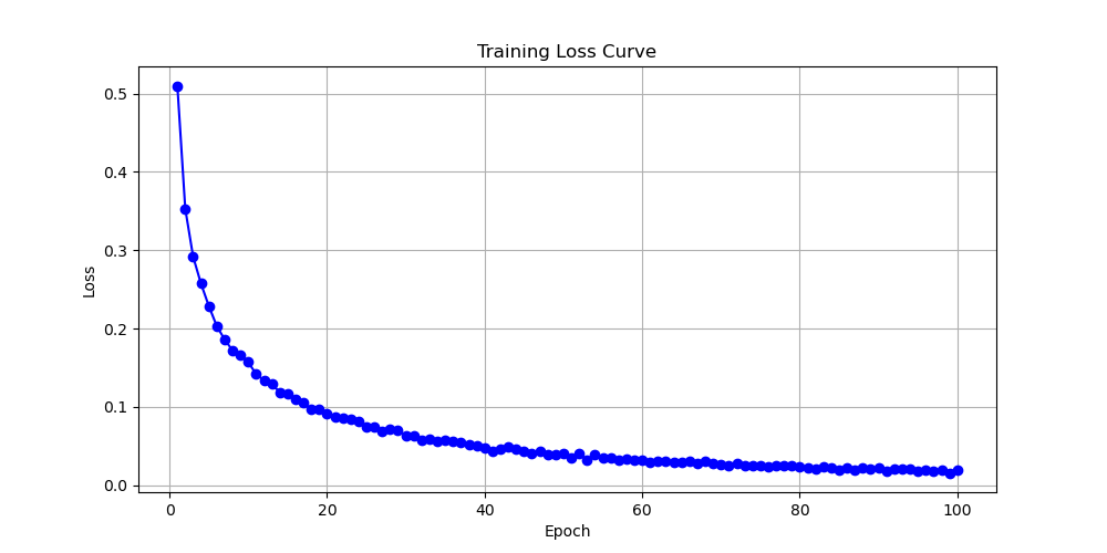
Figure 2. Loss as a function of Epoch for with learning rates of 0.0001, 0.0002, and 0.001 for transformer (Photo/Picture credit: Original).

For the RNN model, after observation, this experiment selected images with learning rates equal to 0.0001, 0.0003, 0.0004, and 0.001. The result shown in Fig. 3 will be presented in the following text. When the learning rate is equal to 0.0001, the final convergence value of the generated loss function image is slightly higher than 0, and the rate of decline is relatively slow. Its performance is considered moderate among these four models. When the learning rate is equal to 0.0003, its loss function converges well towards 0. Its convergence speed is relatively fast. When the epoch is equal to 5, the loss function value is already below 0.2, indicating that the performance of the model is relatively good. When the learning rate is equal to 0.0004, its loss function graph is similar to that when the learning rate is equal to 0.0003. However, the convergence speed of its loss function is slower than that of the previous image with a learning rate equal to 0.0003. Therefore, a model with a learning rate of 0.0004 also performs relatively well. The last image is a loss function graph with a learning rate of 0.001. Its image fluctuation is relatively large, and it does not show a convergence when epoch equals 100. When the model starts running, the function also converges towards 0.1. However, when the epoch reaches 60, the loss function begins to show an upward trend. So, when the learning rate is equal to 0.001, the performance of the model is relatively poor. Comparing these four graphs, it shows that for the process of training MNIST with RNN models, the best learning rate value should be between 0.0003 and 0.0004. The model performance within this range is relatively good, with a fast convergence speed and a final convergence value tending towards 0.

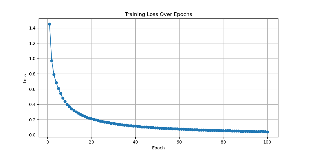
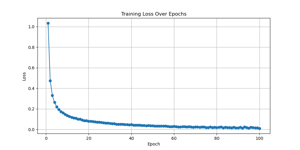
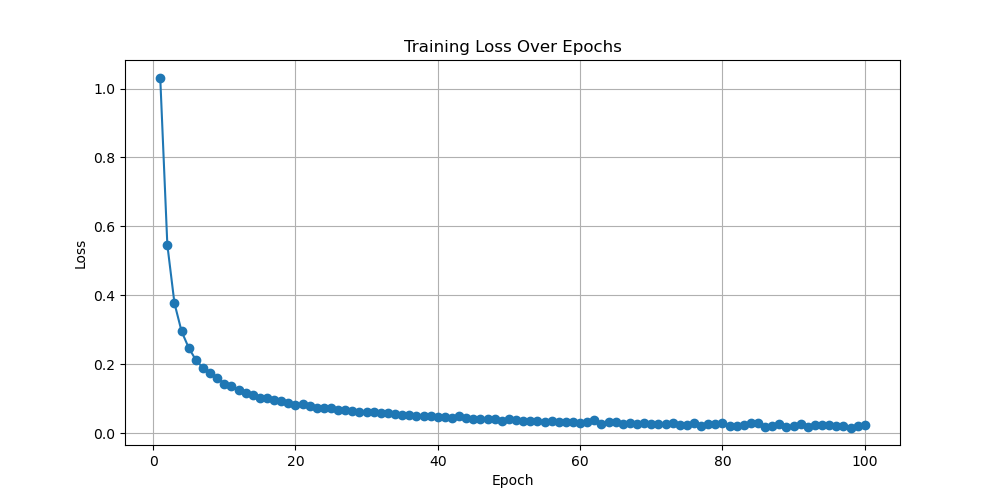
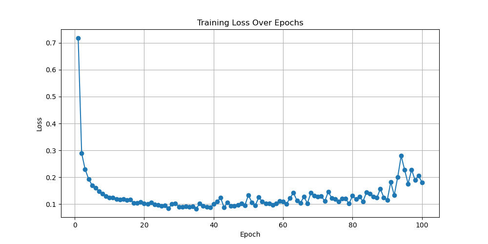
Figure 3. Loss as a function of Epoch with learning rates equal to 0.0001, 0.0003, 0.0004, and 0.001 for RNN (Photo/Picture credit: Original).

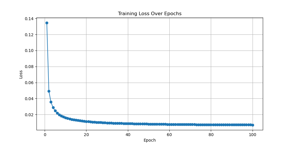
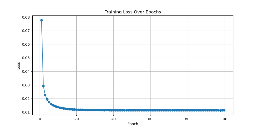
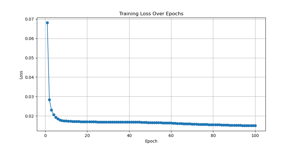
Figure 4. Loss as a function of Epoch with learning rates equal to 0.0001, 0.0005, and 0.001 for diffusion (Photo/Picture credit: Original).

The last model is the diffusion model. This experiment has selected three images with learning rates of 0.0001, 0.0005, and 0.001 for this model. The following text will display the results shown in Fig. 4. The first image has a learning rate of 0.0001, and its convergence speed is relatively fast. When epoch is equal to 100, its convergence value is around 0.1, which is a relatively good convergence graph and the model performance is satisfactory. The second image has a learning rate of 0.0005, which is faster in convergence compared to the first image. The final convergence result is also around 0.1. It is also a model with relatively good performance. The last image is an image with a learning rate equal to 0.001. Its initial value is the smallest, its convergence speed is also the fastest, and the final convergence value is significantly less than 0.1. Therefore, the image with a learning rate of 0.001 has the best convergence among the three images, and its model performance is also the best among these three models. Based on the above three graphs, one cannot confirm which learning rate is the best for training MNIST in the diffusion model. However, one can know that within the learning rate range of 0.0001 to 0.001, the learning rate of 0.001 is the most suitable for training MNIST in diffusion models. For the best learning rate, it should be greater than 0.001and the experiment will test it in the future.

3.2. Explanation of the results

The Transformer, Diffusion, and RNN models are all trained and optimized using the gradient descent algorithm. Although the structures and processes of these three models are not very similar, they all use gradient descent to minimize the loss function. In the process of gradient descent, this study will use this formula \( w^{t+1}=\ w^t\ - \ ∆F(w) \) , where \( \eta \) is the learning rate, \( ∆F(w) \) represents gradient. Learning rate determines the step size for each update. Learning rate plays a significant role in gradient descent, which is why it was set as a variable in the experiment. The following text will explain why the convergence of the loss function also changes when the learning rate changes. Next, this research will discuss the learning rate in three different scenarios. The first situation is that the learning rate is too fast. Excessive learning rate results in excessive step size, which can cause the model to skip the optimal point and fluctuate violently near the optimal solution. This can lead to high-frequency fluctuations or divergence in the loss function image, as shown in the last image of the RNN model, which is caused by excessive learning rate. This situation can lead to unstable convergence of the function graph and the occurrence of oscillations. The second scenario is when the learning rate is too slow. When the learning rate is too low, a small step size can result in slow model updates. At the same time, in this situation, local optima may occur, causing the model to enter local minima and unable to exit these local optima. This can lead to slow convergence and local optima in the model. The third and best scenario is when the learning rate is moderate. In this case, the parameter updates of the model are relatively stable. The loss function graph will gradually converge to a global or local minimum, and the convergence speed is very stable. In theory, this model optimization will gradually approach a stable minimum value.

3.3. Limitations and prospect

For the limitations of this article, there are many factors that affect the convergence of the loss function, and this article only analyzes the learning rate as a hyperparameter. In fact, each hyperparameter has a certain impact on the convergence of the loss function graph, which affects the speed and final convergence value of the loss function graph. Meanwhile, during the range selection process, this experiment only controlled the learning rate between 0.0001 and 0.001, which is a relatively small range. Through the analysis of three models, the transformer model and RNN model can find the optimal learning rate for training MNIST. However, the diffusion model cannot find the optimal learning rate. This is because the optimal learning rate of the diffusion model for training MNIST is greater than 0.001, which is also the limitation of this experiment. One of them is that the influencing factor only takes the learning rate, and the other is that the range of values is too small. For future expectations, it is possible to investigate the impact of more factors on the convergence of the loss function graph and how these factors affect convergence. At the same time, the range of values should be increased and the size of each interval should be reduced. These improvements are aimed at better identifying the optimal hyperparameters for training MNIST with these models. At the same time, this is also an opportunity to search for more datasets, discover how the optimal parameters change between different datasets, and investigate whether the reasons for these changes can be identified. At the same time, it is also possible to search for more models and analyze the different training processes of various models to determine which model training method is better and how to improve this method in order to establish a better model. Various models are constantly improving and perfecting, and one should strive to find better models to promote the development of machine learning and enhance its capabilities.

4. Conclusion

To sum up, the learning rate, as an important hyperparameter, has a significant impact on the convergence of the loss function and deeply affects the performance of a model. When training the MNIST dataset, for the transformer model, a learning rate around 0.0001 shows a performance, while for the diffusion model, a learning rate greater than 0.001 shows a satisfactory performance (due to the issue of hyperparameter interval selection, this experiment did not obtain an interval range). For RNN models, a learning rate between 0.0003 and 0.0004 will exhibit satisfactory convergence performance. For the hyperparameter of learning rate, both too large and too small can lead to poor convergence of the loss function, that is, poor model performance. In the future, more experiments will be conducted on hyperparameters to analyze their impact on the convergence of loss functions, in order to gain a better understanding of model performance. This study analyzes the convergence of the loss function from the hyperparameter of learning rate, which helps these models produce better results in practical applications. Simultaneously, better analyze the significant impact of learning rate on model performance.

References

[1]. Zhong S, Zhang K, Bagheri M, et al 2021 Machine learning: new ideas and tools in environmental science and engineering Environmental science and technology vol 55(19) pp 12741-12754
[2]. Bi Q, Goodman K E, Kaminsky J and Lessler J 2019 What is machine learning? A primer for the epidemiologist American journal of epidemiology vol 188(12) pp 2222-2239
[3]. Shah P, Kendall F, Khozin S, et al 2019 Artificial intelligence and machine learning in clinical development: a translational perspective NPJ digital medicine vol 2(1) p 69
[4]. Vamathevan J, Clark D, Czodrowski P et al 2019 Applications of machine learning in drug discovery and development Nature reviews Drug discovery vol 18(6) pp 463-477
[5]. Kim S J, Cho K J and Oh S 2017 Development of machine learning models for diagnosis of glaucoma PloS one vol 12(5) p e0177726
[6]. Choi R Y, Coyner A S, Kalpathy-Cramer J, Chiang M F and Campbell J P 2020 Introduction to machine learning neural networks and deep learning Translational vision science and technology vol 9(2) pp 14-14
[7]. Carleo G, Cirac I, Cranmer K et al 2019 Machine learning and the physical sciences Reviews of Modern Physics vol 91(4) p 045002
[8]. Morgan D and Jacobs R 2020 Opportunities and challenges for machine learning in materials science Annual Review of Materials Research vol 50(1) pp 71-103
[9]. Athey S and Imbens G W 2019 Machine learning methods that economists should know about Annual Review of Economics vol 11(1) pp 685-725
[10]. Sun S, Cao Z, Zhu H and Zhao J 2019 A survey of optimization methods from a machine learning perspective IEEE transactions on cybernetics vol 50(8) pp 3668-3681
[11]. Vishnu V K and Rajput D S 2020 A review on the significance of machine learning for data analysis in big data Jordanian Journal of Computers and Information Technology vol 6(1)
[12]. Paullada A, Raji I D, Bender E M, Denton E and Hanna A 2021 Data and its (dis) contents: A survey of dataset development and use in machine learning research Patterns vol 2(11)
Cite this article
Fang,X. (2024). Comparison of Convergence for Different Models and Loss Function: Evidence from Transformer, Diffusion and RNN. Applied and Computational Engineering,82,173-180.
Data availability
The datasets used and/or analyzed during the current study will be available from the authors upon reasonable request.
Disclaimer/Publisher's Note
The statements, opinions and data contained in all publications are solely those of the individual author(s) and contributor(s) and not of EWA Publishing and/or the editor(s). EWA Publishing and/or the editor(s) disclaim responsibility for any injury to people or property resulting from any ideas, methods, instructions or products referred to in the content.
About volume
Volume title: Proceedings of the 2nd International Conference on Machine Learning and Automation
© 2024 by the author(s). Licensee EWA Publishing, Oxford, UK. This article is an open access article distributed under the terms and
conditions of the Creative Commons Attribution (CC BY) license. Authors who
publish this series agree to the following terms:
1. Authors retain copyright and grant the series right of first publication with the work simultaneously licensed under a Creative Commons
Attribution License that allows others to share the work with an acknowledgment of the work's authorship and initial publication in this
series.
2. Authors are able to enter into separate, additional contractual arrangements for the non-exclusive distribution of the series's published
version of the work (e.g., post it to an institutional repository or publish it in a book), with an acknowledgment of its initial
publication in this series.
3. Authors are permitted and encouraged to post their work online (e.g., in institutional repositories or on their website) prior to and
during the submission process, as it can lead to productive exchanges, as well as earlier and greater citation of published work (See
Open access policy for details).