1. Introduction

Credit risk management optimization is a continuous pursuit for all financial institutions today. A better risk management system can reduce the bad debt rate of banks while increasing the efficiency of approvals. Nowadays, the number of individuals applying for credit loans from banks is increasing with the continuous social and economic development and people's continuous pursuit of quality of life. The Bank of China's 2023 annual report shows that cumulative credit card issuances rose by 4.22%, and credit card loan balances increased by 8.38% year-on-year [1]. From the above annual report data, it is clear that traditional risk control systems are unable to respond to the growing complexity and diversity of the financial environment, and that traditional risk systems are not able to make good predictions in the face of a large amount of disparate data. Models built through machine learning are more effective and flexible than traditional Risk Control systems which depend on the experience of experts and rule making [2]. A well-developed risk control model can largely reduce unnecessary losses due to credit risk and shorten the waiting time for applicants, which is why major financial institutions are constantly researching machine learning to improve the accuracy of their models [3].

As technology continues to progress, the number of models built through machine learning is countless. Many of the machine learning models have excelled in the area of credit risk control. For example, Classification and Regression Trees (CART) can predict the default probability of a customer based on their historical data and characteristics, and Random Forests (RF) can analyze and then obtain their optimal solution by constructing multiple decision trees, and Support Vector Machines (SVM) can find the optimal decision boundaries in a high-dimensional space and categorize borrowers with different credit risks [4-6]. Orora et al in the study proposed Bootstrap-Lasso (Bolasso) method and applied it to various classification algorithms for comparison and the results concluded that Bolasso's Random Forests algorithms (BS-RF) provide the optimal solution for the purpose of credit evaluation [7]. However, some factors missing from the data set it selected may lead to a decrease in the model's accuracy, such as the number of individuals in the household and the applicant's fixed assets. Lappas and Yannacopoulos offer a unique framework model that optimizes credit risk assessment models by fusing machine learning models with expert knowledge and experience. This approach explores new avenues for improving model accuracy [8]. However, in real practice, this framework may decrease the accuracy of the model because of the subjective bias introduced by the expert's opinion, and the combination of expert knowledge with multiple machine learning models may increase the complexity of the model, resulting in a reduction of the model's maintainability and interpretability in practical applications.

In this paper, different machine learning models were trained on the same dataset and the performance of the models was ranked based on their Comprehensive metrics in order to select a machine learning model most suitable for the risk prediction system. The article is divided into four sections. The first section presented the basic information of the dataset and the experimental protocol. The second section analyzed and discussed the results obtained based on the experimental protocol in the first section. The third part provided a summary of this research.

2. Method

2.1. Data sources and descriptions

The dataset utilized in this paper was obtained from the Kaggle website, and the collectors of its data are labeled according to the real existence of the data, and the applicants mentioned in the dataset are replaced by IDs in consideration of personal privacy. The two datasets that are created from the raw data are called application_record.csv and credit_record.csv. The first dataset contains basic information on 10 feature values for different IDs. The second dataset contains the label values of the data, reflecting the creditworthiness of each ID in different months. The two datasets are inner-joined using IDs. The datasets are first pre-processed, including removing rows with missing values and untrue values, and then all textual data in both datasets are converted to numerical data for machine learning. Before dividing the training and test sets, the percentage of each value in the STATUS column is calculated, with the largest percentage being as high as 98.25% and the smallest being only 0.03%. The quantity and proportion of each category in the original dataset are displayed in Table 1. In order to solve the feature imbalance problem, this paper adopts a custom sampling strategy when dividing the dataset, and the divided datasets are train_data.csv for the training model and test_data.csv for the testing model.

Table 1: Number and percentage of each category in the original dataset

2.2. Selection and description of indicators

The merged dataset has a total of 18 columns of features and 1 column of labels excluding the ID column used for identification. While reading the literature, Sanz et al. found that the combination of SVM and Recursive Feature Elimination (RFE) is very suitable for filtering important features in high dimensional datasets[9]. Han and Kim on the other hand argued that Feature importance (FI) combined with RFE exhibits high robustness in high dimensional datasets and when the data are unbalanced [10]. In order to better filter the important features in this dataset, this paper compared the two methods by mean square error, and the results show that the features filtered by FI+RFE are more important. Table 2 is the definition of each feature column after filtering by FI+RFE.

Table 2: Filtered features and their definitions

2.3. Methodology

For the cleaning of the dataset and the selection of features, the methods have been made above. For the selection of comparison models, RF, SVM, Logistic Regression, Gradient Boosting Decision Trees (GBDT), Gradient Boosting Machine (GBM), and k-Nearest Neighbours (KNN) are selected for comparison. This study will compare the complete metrics to identify the best model and assess the model's performance.

Formulae for RF[11]:

\( \hat{y}=argmax(\sum _{i=1}^{N}I({y_{i}}=c)) \) (1)

Formula for SVM[12]:

\( f(x)=sign(\sum _{i=1}^{N}{α_{i}}{y_{i}}K({x_{i}},x)+b) \) (2)

Formula of Logistic Regression[13]:

\( p(y=1|X)=\frac{1}{1+{e^{-({β_{0}}+\sum _{i=1}^{n}{β_{i}}{x_{i}})}}} \) (3)

Formula of GBDT[14]:

\( {F_{m}}(x)={F_{m-1}}(x)+ν{h_{m(x)}} \) (4)

Formula of GBM[15]:

\( {F_{m}}(x)={F_{m-1}}(x)+ν\cdot {h_{m}}(x) \) (5)

Formula of KNN[16]:

\( \hat{y}=\frac{1}{K}\sum _{i=1}^{k}{y_{i}} \) (6)

3. Results

3.1. Evaluation results

This paper uses extensive measures to evaluate the effectiveness of several machine learning models, such as SVM, GBDT, RF, KNN, GBM, and Logistic Regression, for credit risk assessment. The six models' metrics are shown in Figure 1. With an overall accuracy of 0.71, the Random Forests model outperforms the other models, which are found to perform poorly at medium risk and poorly at no risk, low risk, and high risk. In contrast, SVM has a higher recall of 0.41 in the moderate risk category but reflects the model's lack of ability to discriminate between categories due to its low overall precision and F1-score. The KNN model has an accuracy of 0.69 and performs better in the categories of no risk and high risk, where the model does not discriminate well on moderate risk. The GBM model and the GBDT model similarly demonstrated a lack of recognition ability ( recall of 0) when dealing with medium risk, reflecting the shortcomings of the GBM model and the GBDT model in the prediction of datasets with an unbalanced number of categories. Out of the six models, the logistic regression model had the weakest performance, with an accuracy of only 0.29 while struggling to effectively differentiate between the various risk categories.

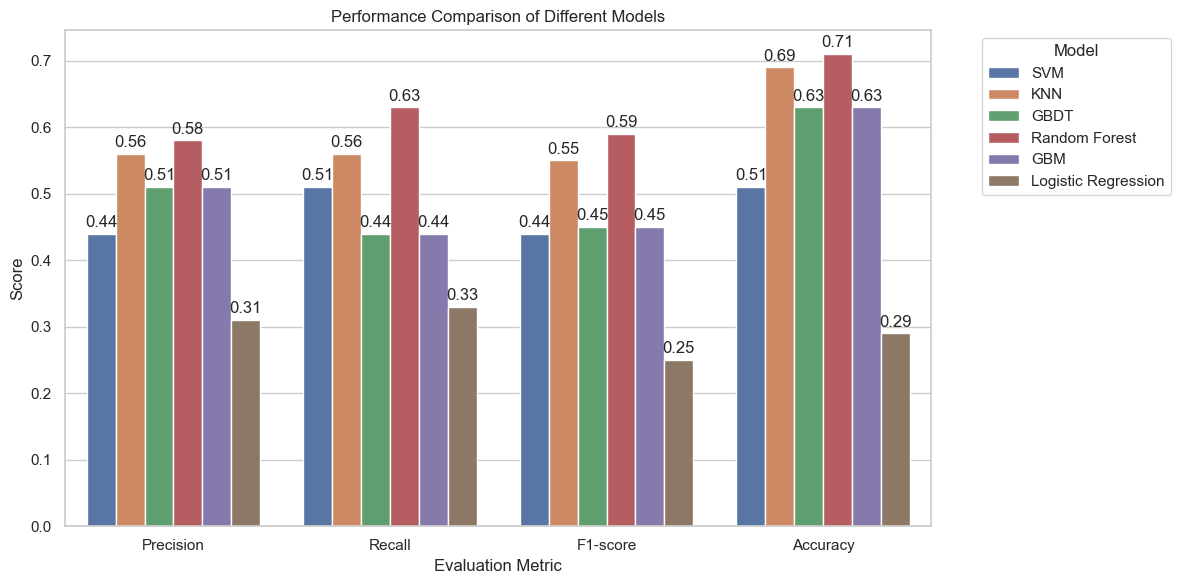
Figure 1: Indicators for each model (F1-score values from macro avg)

3.2. Discussion

In this paper, the RF combined with RFE performed the best in the comparison of the six models. When selecting features, RF is particularly useful in high-dimensional data since it help find the features that are most useful for model prediction. In addition, RF can handle non-linear relationships, which is particularly important in complex datasets. In contrast, RFE enhances the overall accuracy of the model by means of an iterative filtering and removal process of features that do not exert a significant influence on the model's predictions. This ensures that the features employed are of practical value to the training of the model.

In comparison to RF, logistic regression and SVM demonstrate a slight deficiency in their ability to address highly nonlinear risk patterns, due to their inherent limitations in navigating complex relationships. KNN exhibits certain advantages when confronted with low-dimensional datasets. However, it is susceptible to noise interference when dealing with high-dimensional data. GBDT and GBM demonstrate robust recognition capabilities for risk-free categories; however, they exhibit limitations in addressing data imbalance and distinguishing categories with low occupancy.

Figure 2 depicts the confusion matrices for the six models. The matrices can be analyzed to gain insight into the performance of each model across different risk categories. Each model displays a robust capacity to differentiate between the no-risk category and a notable deficiency in its ability to distinguish between medium and high-risk scenarios. The GBDT model is particularly effective in differentiating between the risk-free category and other risk levels. The GBM model demonstrates the greatest efficacy in the prediction of medium risk, likely due to its inherent iterative enhancement mechanism.

Figure 2: Confusion matrix for six models

4. Conclusion

The effectiveness of several machine learning models, such as SVM, KNN, GBDT, RF, GBM, and logistic regression, for assessing credit risk is evaluated in this study. With an overall accuracy of 0.71, the RF paired with the RFE technique shows the most optimal performance, according to a comparison of the models based on precision, recall, F1-score, and accuracy. The model displays a balanced performance across all risk categories, with an average precision across these categories that is the highest of the six models.

Although this paper identifies the advantages of the RF+RFE combination, it is also constrained by the limited number of 'medium-risk categories in the sample, which restricts the model's capacity to identify this category. Thus, expanding the dataset or incorporating data enhancement methods like Generative Adversarial Networks may be addressed in future studies to enhance the model's prediction capacity for a few categories.

Taken together, the study's findings show that, in terms of machine learning models, the RF model is the most effective at assessing credit risk. It is a useful tool for managing financial risk due to its strong feature set and capacity to handle uneven data. Future research could further extend the dataset types and introduce more advanced modeling techniques to further improve the performance and practical application value of the models. Regarding the potential use of machine learning models in credit risk assessment, the findings of these studies offer insightful references.

References

[1]. Bank of China.2023 Annual Report.March 28, 2024. Retrieved on August 27, 2024. Retrieved from:https://www.boc.cn/investor/ir3/202403/t20240328_24820135.html
[2]. Shi, S., Tse, R., Luo, W., D’Addona, S., & Pau, G. (2022). Machine learning-driven credit risk: a systemic review. Neural Computing and Applications, 34(17), 14327-14339.
[3]. Ghazieh, L., & Chebana, N. (2021). The effectiveness of risk management system and firm performance in the European context. Journal of Economics, Finance and Administrative Science, 26(52), 182-196.
[4]. Lewis, R. J. (2000, May). An introduction to classification and regression tree (CART) analysis. In Annual meeting of the society for academic emergency medicine in San Francisco, California (Vol. 14). San Francisco, CA, USA: Department of Emergency Medicine Harbor-UCLA Medical Center Torrance.
[5]. Breiman, L. (2001). Random forests. Machine learning, 45, 5-32.
[6]. Jakkula, V. (2006). Tutorial on support vector machine (SVM). School of EECS, Washington State University, 37(2.5), 3.
[7]. Arora, N., & Kaur, P. D. (2020). A Bolasso based consistent feature selection enabled random forest classification algorithm: An application to credit risk assessment. Applied Soft Computing, 86, 105936.
[8]. Lappas, P. Z., & Yannacopoulos, A. N. (2021). A machine learning approach combining expert knowledge with genetic algorithms in feature selection for credit risk assessment. Applied Soft Computing, 107, 107391.
[9]. Sanz, H., Valim, C., Vegas, E., Oller, J. M., & Reverter, F. (2018). SVM-RFE: selection and visualization of the most relevant features through non-linear kernels. BMC bioinformatics, 19, 1-18.
[10]. Han, S., & Kim, H. (2021). Optimal feature set size in random forest regression. Applied Sciences, 11(8), 3428.
[11]. Breiman, L. (2001). Random forests. Machine learning, 45, 5-32.
[12]. Hearst, M. A., Dumais, S. T., Osuna, E., Platt, J., & Scholkopf, B. (1998). Support vector machines. IEEE Intelligent Systems and their applications, 13(4), 18-28.
[13]. Wright, R. E. (1995). Logistic regression.
[14]. Ke, G., Meng, Q., Finley, T., Wang, T., Chen, W., Ma, W., ... & Liu, T. Y. (2017). Lightgbm: A highly efficient gradient-boosting decision tree. Advances in neural information processing systems, 30.
[15]. Natekin, A., & Knoll, A. (2013). Gradient boosting machines, a tutorial. Frontiers in neurorobotics, 7, 21.
[16]. Peterson, L. E. (2009). K-nearest neighbor. Scholarpedia, 4(2), 1883.
Cite this article
Han,B. (2024). Evaluating Machine Learning Techniques for Credit Risk Management: An Algorithmic Comparison. Applied and Computational Engineering,112,29-34.
Data availability
The datasets used and/or analyzed during the current study will be available from the authors upon reasonable request.
Disclaimer/Publisher's Note
The statements, opinions and data contained in all publications are solely those of the individual author(s) and contributor(s) and not of EWA Publishing and/or the editor(s). EWA Publishing and/or the editor(s) disclaim responsibility for any injury to people or property resulting from any ideas, methods, instructions or products referred to in the content.
About volume
Volume title: Proceedings of the 5th International Conference on Signal Processing and Machine Learning
© 2024 by the author(s). Licensee EWA Publishing, Oxford, UK. This article is an open access article distributed under the terms and
conditions of the Creative Commons Attribution (CC BY) license. Authors who
publish this series agree to the following terms:
1. Authors retain copyright and grant the series right of first publication with the work simultaneously licensed under a Creative Commons
Attribution License that allows others to share the work with an acknowledgment of the work's authorship and initial publication in this
series.
2. Authors are able to enter into separate, additional contractual arrangements for the non-exclusive distribution of the series's published
version of the work (e.g., post it to an institutional repository or publish it in a book), with an acknowledgment of its initial
publication in this series.
3. Authors are permitted and encouraged to post their work online (e.g., in institutional repositories or on their website) prior to and
during the submission process, as it can lead to productive exchanges, as well as earlier and greater citation of published work (See
Open access policy for details).