


1.Introduction
The Support Vector Machine (SVM) is a supervised learning model initially developed based on the research by Soviet scholars Vladimir N. Vapnik and Alexander Y. Lerner in 1963. It is commonly used for pattern recognition, classification, and regression analysis, serving as a widely applied discriminative method in the field of machine learning. In 1992, Bernhard E. Boser, Isabelle M. Guyon, and Vapnik introduced kernel methods, enabling SVMs to handle non-linearly separable data [1].
The SVM algorithm essentially solves a quadratic programming problem. When dealing with large-scale sample data, the number of matrix elements grows quadratically with the size of the training set. In 2014, P. Rebentrost et al. proposed the Quantum Support Vector Machine (QSVM) [2]. The QSVM transforms the quadratic programming problem of SVMs into a least squares problem and leverages quantum algorithms to efficiently solve key steps such as vector inner products, thereby significantly reducing computational complexity. Compared to classical SVMs, QSVMs have significant advantages in computational efficiency, especially when dealing with large-scale datasets, where the complexity is reduced exponentially.
Since 1995, when Professor Kak of Louisiana State University proposed the concept of quantum neural computing, the theoretical and applied research on quantum computing acceleration has gradually gained popularity. In 2001, Horn et al. introduced a new clustering algorithm based on quantum mechanics for unsupervised clustering. In 2009, Harrow et al. proposed the famous HHL algorithm, which achieved exponential speedup compared to the best-known classical algorithm with a time complexity ofO(n)[3].
Although many scholars have conducted research on the time complexity and practical applications of quantum support vector machines and made outstanding contributions to the direction of quantum computing, there are still issues of low accuracy and large approximation values in unitary matrix simulations, and the feature dimension of the training dataset is only two-dimensional.
To apply quantum support vector machines in multi-feature dimensional non-linear data spaces, this paper designs a computational architecture combining classical and quantum computing. It utilizes Pauli decomposition of Hermitian matrices to simulate the quantum simulation of Hamiltonians. Based on the HHL algorithm, quantum phase estimation, quantum Fourier transform, and conditional rotation transformations of quantum states are designed to construct a quantum circuit for solving linear equations and realize the quantum simulation of unitary operators[4].
2.Quantum Algorithm Design
To solve the equationAx=bfor a given Hermitian matrixA∈RN×Nand a vector→b∈RNon a quantum computer using the HHL algorithm, the first step is to perform quantum state encoding. Assuming the dimension of the Hermitian matrixAisN=2n, wherenis the number of quantum bits used for quantum state encoding. For vectors→band→x, during quantum state encoding, the i-th element of 𝑏 (or 𝑥) is encoded as the i-th basis state of the quantum superposition state |𝑏⟩ (or |𝑥⟩). Through a quantum circuit, the solution satisfying A|𝑥⟩ = |𝑏⟩ is obtained[5].
The HHL algorithm circuit design mainly consists of three modules: quantum phase estimation, controlled rotation of quantum states, and quantum state inversion and calculation.
2.1.Principle of the HHL Algorithm
Given a Hermitian matrixAand a vector→b, suppose the spectral decomposition ofAis as follows:A=∑Nj=1λj|uj⟩⟨uj| (1)
Express|b⟩in terms of the basis{|uj⟩}:|b⟩=∑Nj=1βj|uj⟩. Using quantum phase estimation (QPE) withU=eiAΔt, the result is as follows:
|b⟩→∑Nj=1βj|uj⟩| λj⟩ (2)
For equation (2), applying operatorUyieldseiAΔt=∑Nj=1eiλjΔt|uj⟩⟨uj|, where| λj⟩represents an estimate of the eigenvalueλj(the wavy line indicates an estimate, the same applies to the following). The solution to the equation is:|x⟩=A−1|b⟩=∑jβj(λj)−1|uj⟩ (3)
The key of the algorithm is to simulate the operatorU=eiAΔton|b⟩, which will be described in detail later.
2.2.Data preprocessing and quantum state encoding
In the HHL algorithm, matrixAis required to be Hermitian, that is, matrixAneeds to satisfyA†=A, this requirement can be relaxed in the concrete implementation, ifAis not Hermitian, construct Aas follows:
A=(0AA†0) (4)
Then solving the equation A→y=(→b0), it is verified that the solution→yof the obtained equation must have the form→y=(0→x), whereA→x=→b. Because the HHL algorithm is a quantum algorithm, the vector→bneeds to be encoded into the quantum state and input in the quantum state|b⟩.
One of the keys of the HHL algorithm is the quantum state encoding of vectors and matrices, and the target register is set to store the information of quantum state|b⟩. The initial state of the quantum state is|0⟩⊗n, that is, all qubits are in the|0⟩state, and the value of the vector→bis encoded to|b⟩to satisfy|b⟩=∑Ni=1bi|i⟩ (5)
Wherebiis the i-th component of vectorband∑i|bi|2=1.
In the concrete implementation, the rotation gate is used to encode the components of the vector into the amplitude of the qubit. As shown in Figure. 1, using a rotation gate, the quantum state is rotated from|0⟩to the target state related to the Angleθ. The amplitude is encoded by adjusting the rotation Angle. The rotation Angleθis calculated based on the inverse trigonometric function of the amplitude:θ=2×arcsin(bi) (6)
After rotation, the amplitude of each qubit has been associated with the corresponding component of vector→b, and the quantized representation|b⟩of vector→bis obtained[6].
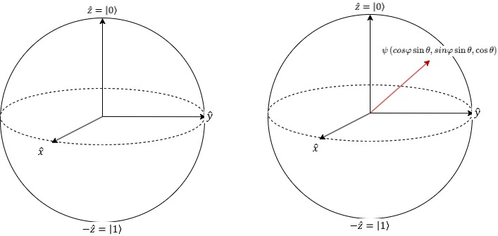
Figure 1: Quantum states are encoded on the Bloch sphere
2.3.Quantum phase estimation
For a unitary matrixU, which has a complex eigenvalueeiφand an eigenvector|u⟩with a modulus of 1, the purpose of the quantum phase estimation algorithm is to estimate the value of the phaseφwithin a certain error range[7].
In this paper, the unitary operatorU=ei2πAcorresponding to matrixAhas an eigenvalueei2πλand an eigenvector|u⟩, where|u⟩is the eigenvector of the real eigenvalueλofA.
The steps of phase estimation can be divided into three steps. Firstly, Hadamard gate operation is performed on all qubits of the phase register, and controlledUgate operation is performed continuously on the control register, where the power ofUgate is20,21,…,2t−1, the control bits areqt−1,qt−2,…,q1,q0, then the state in the first register is going to be
|ψ1⟩=12t2(|0⟩+ei2π2t−1φ|1⟩)(|0⟩+ei2π2t−2φ|1⟩)…(|0⟩+ei2π20φ|1⟩)
That is
|ψ1⟩=12t2∑2t−1k=0ei2πφk|k⟩ (7)
Wherekis the decimal representation of the tensor product state.
Subsequently, an inverse quantum Fourier transform is applied to the phase register, denoted asQFT†in the circuit. Applying the inverse quantum Fourier transform to|ψ1⟩yields|ψ2⟩[8].
|ψ2⟩=QFT†|ψ1⟩=12t∑2t−1x=0ax|x⟩ (8)
Whichax=∑2t−1k=0e2πik(φ−x/2t)for eigen vector|x⟩(x=0.1,...,2t). According to the above equation, when2tφis an integer andx=2tφis satisfied, the probability amplitude is the maximum value 1, and the final state of the first register can accurately reflectφ. When2tφis not an integer,xis an estimate ofφ, and the largertis, the more accurate the estimate will be.
Finally, the quantum bit of the first register was measured, and the final state of the first registerf=∑2t−1xax|x⟩,x=0,1,...,2t, from which the largest amplitudeamaxis found, and the corresponding intrinsic basis vector|x⟩inxdivided by2tis the estimated value of the phase.
Overall, when usingtauxiliary qubits, the effect of QPE can be written as follows.|b⟩|0⟩⊗t|0⟩=∑Nj=1βj|uj⟩|0⟩⊗t|0⟩→∑Nj=1βj|uj⟩| φj⟩|0⟩ (9)
2.4.Conditional rotation
After QPE, available quantum state∑Nj=1βj|uj⟩| φj⟩|0⟩, To extract the information ofλjfrom the quantum state| φj⟩, the specific implementation using the controlled rotation gateCR(k)is as follows:
CR(k)| φ⟩|b⟩={| φ⟩|b⟩,k≠ φ| φ⟩Ry(2arcsinCλ)|b⟩,k= φ (10)
Whenkchooses the correct φ, the selection operation will be applied to the subsequent qubits. Since the correct φis not yet known, a brute force enumeration of all possibleCR(k)is used, and the specific effect is as follows:∏2t−1k=1I⊗CR(k)∑Nj=1βj|uj⟩| φj⟩|0⟩=∑Nj=1βj|uj⟩| φj⟩(√1−(Cλj)2|0⟩+Cλj|1⟩) (11)
Applying the inverse QPE once more, the overall quantum state is as follows:|ψ⟩=∑Nj=1βj|uj⟩|0⟩⊗t(√1−(Cλj)2|0⟩+Cλj|1⟩) (12)
2.5.Framework of quantum circuits
The overall framework of HHL is shown in Figure 2. qc defines the qubits used for QPE, qb defines the qubits representing vector→b. In order to make the quantum circuit structure clear, QPE and controlled selection module are encapsulated here (quantum phase estimation is a unitary operation in general, and quantum phase inversion part can be obtained by QPE module mirror).
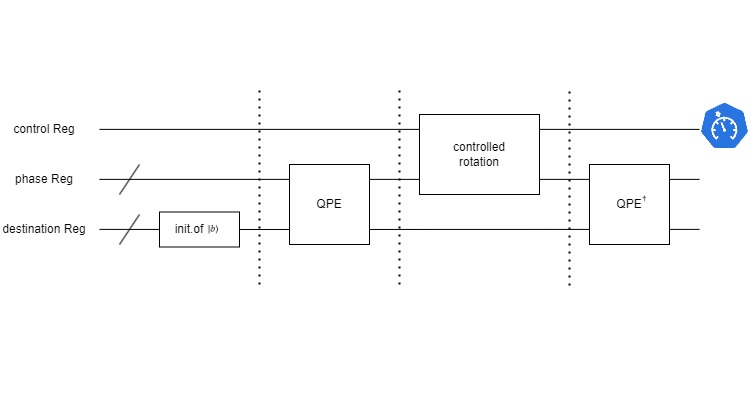
Figure 2: Quantum linear Computing Circuit
The framework of quantum phase estimation is shown in Figure. 3, QFT is the encapsulation of inverse quantum Fourier transform, andUjrepresents the controlledUjoperation of the target register with the quantum bits in the phase register as the control bits one by one.
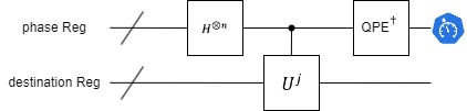
Figure 3: Quantum phase Estimation circuit
In the HHL algorithm, the goal of controlled unitary operation is to realize the time evolutione−iAtof matrixA, and extract its eigenvalues through quantum phase estimation. This process depends on the controlled relationship between the control qubit and the target quantum state. In this paper, the time evolution of matrix is simulated by controlled Z rotation gate (CRZ). For matrixA, the quantum state is evolved in time as follows:
U(t)=e−iAt (13)
This is the evolution ofAquantum state under the action of a matrixA, wheretis a time parameter and i is an imaginary unit. To extract the eigenvalues from the matrixA, different powers of this time evolution operator are applied in the quantum phase estimation step:Uj=e−iAtj, wheretjis the time step corresponding to the phase estimation qubit. In a quantum circuit, the controlled unitary operation needs to apply different times ofUjaccording to the state of the control qubit.CRZis used to approximately realize this operation. The function ofCRZ(θ)is to perform a Z-axis rotation of the target quantum state with a rotation Angle ofθ, which can be expressed as follows:
CRZ(θ)=(101eiθ) (14)
Where the rotation Angleθ=−2dtis related to the time stepdt, and the phase information associated with the matrixAis gradually accumulated through2icontrolled rotations. This phase information is subsequently decoded via an inverse quantum Fourier transform to extract matrix eigenvalues, which are ultimately used to solve linear systems of equations.
3.Multi-dimensional nonlinear feature space processing
When dealing with multi-dimensional nonlinear feature data, to avoid the high memory occupation and computational complexity caused by the explicit calculation of feature vectors in high-dimensional space. In this paper, the kernel method is used to map the data from the original space to a high-dimensional feature space, which is achieved by computing the kernel matrix. Each element of the kernel matrix represents the inner product between two samples in high-dimensional space. In this paper, Using the linear kernel functionK(xi,xj)=xi∙xjand radial basis function (RBF kernel)K(xi,xj)=exp(−||xi−xj||22σ2)process of linear and nonlinear can be divided into data respectively. Whereσis a parameter that controls the width of the RBF kernel.
The kernel matrixKis derived by calculating the similarity between samples, and each elementKijrepresents the inner product of the training samplesxiandxjin a high-dimensional feature space, without explicitly calculating the coordinates of the whole high-dimensional space. Suppose the samples in the training set are{x1,x2,x3…xn}, eachxiis ad-dimensional vector, and the kernel matrixKis anN×Nsymmetric matrix whose entriesKijare defined by
Kij=ϕ(xi)Tϕ(xj) (15)
Whereϕis a mapping function from the original input space to a high-dimensional feature space, and the kernelK(xi,xj)is defined as follows:K(xi,xj)=〈ϕ(xi),ϕ(xj)〉 (16)
The kernel function can compute the inner product of two samples in the high-dimensional feature space without explicitly constructing the mappingϕ. For each pair of samples(xi,xj),K(xi,xj)is calculated through the kernel function, and the corresponding positionKijof the kernel matrix is filled to complete the calculation of the kernel matrixK[9].
4.Implementation of support vector machine calculation acceleration
After kernel method mapping, the data that cannot be linearly classified in the original space can be found in a linearly separable hyperplane in the high-dimensional feature space. However, with the growth of the data set, the computational complexity of the kernel matrix increases rapidly in the face of large sample size and high-dimensional features, which brings significant computational overhead. In order to cope with this problem, this paper proposes to introduce quantum computing to accelerate the calculation of kernel matrix, and use the HHL algorithm to significantly accelerate the linear system solution.
Using the property of quantum coherent superposition, for solving the linear equation system of kernel matrixK:Kα=b, whereKis the kernel matrix,αis the Lagrange multiplier, andbis the polarization term. Compared with the classical solution, the time complexity grows polynomial-ly with the increase of the number of samples, which is usuallyO(n3)level, the quantum computing acceleration reduces the complexity to the exponential level, namelyO(logn).
Firstly, the kernel matrixKis calculated by the kernel method, and the matrixKand vector→bare encoded into quantum states|k⟩and|b⟩. Through quantum phase estimation, the eigenvalue information of matrixKis obtained by the HHL algorithm, so as to invert the matrix. The algorithm constructs the inverse of the matrix by reverse operation, and finally obtains the quantum state representation ofα
|α⟩=K−1|b⟩ (17)
By decoding the quantum states, the corresponding solution can be obtained. It greatly improves the efficiency of solving the kernel matrix in the classical SVM, especially in the processing of large-scale high-dimensional data.
5.Experimental results and analysis
5.1.Error analysis
In the HHL algorithm, the time evolutione−iAtis approximately realized by the controlled revolving gateCRZ, which can only be approximated infinitely. In this study, the approximation error is specified as follows:
In terms of the approximation error of the discrete time evolution, since the time evolution of the matrix cannot be directly and accurately realized, this study approximates the simulation by a series of discrete controlled rotation gates. Each time theCRZgate is applied, the actual rotation performed by the system is a discrete time step dt. The step size of the time evolution operator is as follows: U(t)={e^{-iAt}}≈\prod _{j=1}^{N}{e^{-iA∆t}}\ \ \ (18)
Approximation error analysis For dt , the Taylor series expansion of Equation (18) is carried out to evolve in n time steps, and the overall evolution operator is as follows: U(t)=I-iAt+\frac{{(-iAdt)^{2}}}{2}n+O({(dt)^{3}}) , where n=\frac{t}{dt} , the approximation error mainly comes from the higher order terms, then the approximation error of the time evolution operator can be obtained as follows: {ϵ_{U}}=\frac{{t^{2}}}{2}{‖A‖^{2}}∙\frac{1}{{(dt)^{2}}}\ \ \ (19)
Where ∆t=\frac{t}{N} is the time step is the number of steps. This discretization introduces an error proportional to the step size ∆t , typically O(∆{t^{2}}) . If the number of time steps N is large enough, the error can become small, but at the same time it will increase the circuit depth and complexity.
The approximation of the time evolution depends on the range of eigenvalues of the matrix A . If the eigenvalue {λ_{i}} of matrix A has a large span, the error will be amplified. The larger the eigenvalue is, the faster the change of the phase factor {e^{-i{λ_{i}}t}} in the time evolution operator, and the discrete-time evolution approximation of these phases will produce large errors. The relationship between the estimated error and the eigenvalue size is as follows:
{ϵ_{λ}}=\frac{∆t}{{λ_{max}}}\ \ \ (20)
Where {λ_{max}} is the largest eigenvalue of matrix A . When the eigenvalues are large, a smaller time step ∆t is required to keep the error small.
The accuracy of quantum phase estimation is limited by the number of QPE qubits. QPE performs phase estimation through finite number of qubits, and the estimation accuracy is proportional to the number of qubits t . If t qubits are used, the error in phase estimation is as follows:
{ϵ_{QPE}}=\frac{2π}{{2^{t}}}\ \ \ (21)
In the concrete implementation, the CRZ controlled rotation gate itself may be affected by hardware implementation errors and noise. On practical quantum hardware, the precision of gate operation may lead to additional errors due to noise and imprecision of gate operation.
Considering the above errors, the total error of the HHL algorithm can be approximately expressed as follows:
{ϵ_{total}}={ϵ_{U}}+{ϵ_{λ}}+{ϵ_{QPE}}\ \ \ (22)
The total error depends on the number of time steps N , the number of qubits t , the range of matrix eigenvalues, and the specific hardware noise. If the number of qubits t used is small or the eigenvalue {λ_{max}} is large, a finer time step or more QPE qubits are needed to reduce the error.
5.2.Dataset and experimental results
In this study, the classification performance of QSVM was compared with SVM in a multidimensional nonlinear feature space. The paper used the Iris dataset, which contains 150 samples covering three species of iris (Iris mountain, Iris variatum, and Iris Virginia) with 50 samples per species[10]. Three dimensional, four dimensional, five dimensional and six dimensional feature subsets are extracted for testing. The three dimensional features include calyx length, calyx width and petal length, and the other dimensions add petal width features to evaluate the influence of different dimensions on the classification effect. Due to the bottleneck of quantum computing hardware technology, the linear solution has stability problems, so the ratio of calculation accuracy to calculation time is used as the index for performance evaluation. Using IBM qiskit development platform[11]. The model performance is shown in Figure 4:
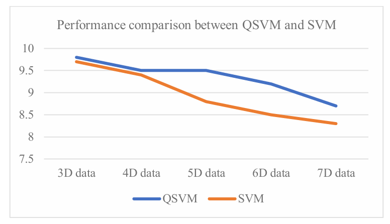
Figure 4: Performance data
The experimental results show that the classification accuracy of QSVM is generally higher than that of classical SVM on these data sets. In particular, when handling high-dimensional and nonlinear features, QSVM demonstrates superior classification capabilities. In terms of computation time and memory requirements, QSVM shows significant advantages, especially when dealing with large-scale datasets.
6.Conclusion
In this paper, the acceleration method of quantum computing for SVM in multi-dimensional nonlinear feature space is studied, and a new algorithm combining the advantages of classical and quantum computing is proposed. Experimental results show that QSVM outperforms classical SVM in terms of classification performance, computation time and memory requirements. However, the practical application of quantum computing still faces numerous challenges, including the maturity of quantum hardware and the correction of quantum errors. Future research can further explore more efficient quantum mapping algorithms and quantum circuit optimization methods to improve the performance and practicability of QSVM.
References
[1]. Boser, B. E., Guyon, I. M., & Vapnik, V. N. (1992). A training algorithm for optimal margin classifiers. In COLT '92: Proceedings of the fifth annual workshop on Computational learning theory.
[2]. Rebentrost, P., Mohseni, M., & Lloyd, S. (2014). Quantum Support Vector Machine for Big Data Classification. Physical Review Letters, 113(13), 130503.
[3]. Aram, W. H., Avinatan, H., Seth, L. (2008). Quantum algorithm for solving linear systems of equations. Quantum Physics.
[4]. Wang, Y., Li, G., & Wang, X. (2023). A hybrid quantum-classical Hamiltonian learning algorithm. Science China (Information Sciences), 66(2), 295-296.
[5]. Yue, T., Wu, C., Liu, Y., Du, Z., Zhao, N., Jiao, Y., Xu, Z., & Shi, W. (2023). HASM quantum machine learning. Science China (Earth Sciences), 66(9), 1937-1945.
[6]. Wang, S., Zhang, K., & Zhang, L. (2020). Research on the decomposition of unitary operators in quantum circuits. Natural Science Journal of Heilongjiang University, 37(6), 653-660.
[7]. Papadopoulos, N. J. C., Reilly, J. T., Wilson, J. D., & Holland, M. J. (2024). Reductive quantum phase estimation. Physical Review Research, 6(3), 033051.
[8]. Wong, H. Y. (2023). Quantum Fourier Transform I. In Introduction to Quantum Computing (pp. 243-253).
[9]. Pedrycz, W. (2002). Advances in Kernel Methods. Support Vector Learning, by B. Scholkopf, C. J. C. Burges, and A. J. Smola. Neurocomputing, 47(1), 303-304. ISBN 0-262-19416-3.
[10]. Dua, D. and Graff, C. (2019). Iris Data Set. UCI Machine Learning Repository. Available at: https://archive.ics.uci.edu/ml/datasets/iris
[11]. Javadi-Abhari, A., Treinish, M., Krsulich, K., Wood, C. J., Lishman, J., Gacon, J., Martiel, S., Nation, P. D., Bishop, L. S., Cross, A. W., Johnson, B. R., & Gambetta, J. M. (2024). Quantum computing with Qiskit.
Cite this article
Liu,H. (2024). Research on Quantum Computing Acceleration of Support Vector Machines in Multi-dimensional Nonlinear Feature Spaces. Applied and Computational Engineering,100,100-109.
Data availability
The datasets used and/or analyzed during the current study will be available from the authors upon reasonable request.
Disclaimer/Publisher's Note
The statements, opinions and data contained in all publications are solely those of the individual author(s) and contributor(s) and not of EWA Publishing and/or the editor(s). EWA Publishing and/or the editor(s) disclaim responsibility for any injury to people or property resulting from any ideas, methods, instructions or products referred to in the content.
About volume
Volume title: Proceedings of the 5th International Conference on Signal Processing and Machine Learning
© 2024 by the author(s). Licensee EWA Publishing, Oxford, UK. This article is an open access article distributed under the terms and
conditions of the Creative Commons Attribution (CC BY) license. Authors who
publish this series agree to the following terms:
1. Authors retain copyright and grant the series right of first publication with the work simultaneously licensed under a Creative Commons
Attribution License that allows others to share the work with an acknowledgment of the work's authorship and initial publication in this
series.
2. Authors are able to enter into separate, additional contractual arrangements for the non-exclusive distribution of the series's published
version of the work (e.g., post it to an institutional repository or publish it in a book), with an acknowledgment of its initial
publication in this series.
3. Authors are permitted and encouraged to post their work online (e.g., in institutional repositories or on their website) prior to and
during the submission process, as it can lead to productive exchanges, as well as earlier and greater citation of published work (See
Open access policy for details).
References
[1]. Boser, B. E., Guyon, I. M., & Vapnik, V. N. (1992). A training algorithm for optimal margin classifiers. In COLT '92: Proceedings of the fifth annual workshop on Computational learning theory.
[2]. Rebentrost, P., Mohseni, M., & Lloyd, S. (2014). Quantum Support Vector Machine for Big Data Classification. Physical Review Letters, 113(13), 130503.
[3]. Aram, W. H., Avinatan, H., Seth, L. (2008). Quantum algorithm for solving linear systems of equations. Quantum Physics.
[4]. Wang, Y., Li, G., & Wang, X. (2023). A hybrid quantum-classical Hamiltonian learning algorithm. Science China (Information Sciences), 66(2), 295-296.
[5]. Yue, T., Wu, C., Liu, Y., Du, Z., Zhao, N., Jiao, Y., Xu, Z., & Shi, W. (2023). HASM quantum machine learning. Science China (Earth Sciences), 66(9), 1937-1945.
[6]. Wang, S., Zhang, K., & Zhang, L. (2020). Research on the decomposition of unitary operators in quantum circuits. Natural Science Journal of Heilongjiang University, 37(6), 653-660.
[7]. Papadopoulos, N. J. C., Reilly, J. T., Wilson, J. D., & Holland, M. J. (2024). Reductive quantum phase estimation. Physical Review Research, 6(3), 033051.
[8]. Wong, H. Y. (2023). Quantum Fourier Transform I. In Introduction to Quantum Computing (pp. 243-253).
[9]. Pedrycz, W. (2002). Advances in Kernel Methods. Support Vector Learning, by B. Scholkopf, C. J. C. Burges, and A. J. Smola. Neurocomputing, 47(1), 303-304. ISBN 0-262-19416-3.
[10]. Dua, D. and Graff, C. (2019). Iris Data Set. UCI Machine Learning Repository. Available at: https://archive.ics.uci.edu/ml/datasets/iris
[11]. Javadi-Abhari, A., Treinish, M., Krsulich, K., Wood, C. J., Lishman, J., Gacon, J., Martiel, S., Nation, P. D., Bishop, L. S., Cross, A. W., Johnson, B. R., & Gambetta, J. M. (2024). Quantum computing with Qiskit.