1. Introduction

SLAM functionalities have importantly been improved with the arrival of 5G technology, introducing communication at high speed and low latency. Considering that SLAM is important in such fields as robot navigation, autonomous driving, unmanned logistics, and IoV, real-time navigation of vehicles at an obstruction-avoiding distance is guaranteed and, consequently, the support in warehouse drawing necessary for delivery accuracy. SLAM further enhances the structuring and transportation in IoT of Vehicles, improving safety and efficiency in the management of transport.

The technology of simultaneous localization and map construction was born in 1980s, which solved the problem of autonomous localization and map construction of robots in unknown environment [1]. In recent years, with the development of computing power, sensor technology and algorithm, SLAM system has made remarkable progress. For example, ORB-SLAM is a feature-based visual SLAM method, which is suitable for monocular, stereo, and RGB-D cameras. It makes key frame selection, location, and map construction [2] through ORB features, and reduces the dependence on lidar through visual sensors, making the system more economical and portable [3]. In addition, direct SLAM methods, such as LSD-SLAM, directly use pixel brightness information for image registration without extracting feature points [4]. However, SLAM system, especially the system based on point cloud data, still faces some challenges, such as environmental reflectivity [5] and transient map [6] caused by moving objects will cause a decline of the accuracy of lidar data, which will lead to the instantaneity of the map. In the absence of obvious features, point cloud registration may mislead the algorithm and lead to “position loss” [7].

As an indispensable part of SLAM, ICP algorithm achieves optimal overlap by registering two groups of 3D point clouds [8]. This algorithm achieves accurate registration by iteratively finding corresponding points, calculating the optimal rigid body transformation matrix, and minimizing the sum of squares of errors. Although ICP faces the challenge of large amount of calculation and strong dependence on initial estimation when dealing with large-scale complex scenes, its accuracy is enough to meet the needs of most modern SLAM systems [8]. There are two main variants of ICP algorithm: point-to-point and point-to-plane Point-to-point ICP matches each point in the source point cloud with the nearest point in the target point cloud, but it may converge slowly in complex shapes and be sensitive to noise [9,10]. Point-to-plane ICP introduces surface normal to minimize errors, but it requires accurate normal calculation, which may be unstable in sparse or low-density point clouds [11,12]. In order to overcome the limitations of ICP algorithm in complex environment, this paper proposes an improved algorithm, which optimizes the registration process by dynamically adjusting the number of iterations, thus improving its accuracy in various application scenarios.

2. ICP Algorithm and Its Limitations

The core of Iterative Nearest Point (ICP) algorithm is to achieve optimal registration by minimizing the distance between two point clouds, that is, given two point clouds P and Q. The goal of ICP algorithm is to find an optimal transformation (including rotation and translation) to minimize the distance between the transformed point cloud P and the point cloud Q. This can be calculated in Eq. (1):

\( E(R,t)=\sum _{i=1}^{N}|R\cdot {P_{i}}+t-{Q_{i}}{|^{2}}\ \ \ (1) \)

Here \( R \) stands for rotation matrix, \( t \) stands for translation vector, and \( {P_{i}} \) and \( {Q_{i}} \) are the corresponding points in point clouds \( P \) and Q.

Although ICP algorithm shows powerful functions in many applications, it also faces some limitations when dealing with complex environments, especially in the case of partial overlap, noise and poor initial alignment, the performance of ICP algorithm will be significantly affected. These limitations are mainly due to the fixed iterative mechanism of the algorithm, which cannot be adjusted adaptively according to the change of environmental complexity. This study will explain in detail the reasons for these limitations:

2.1. Convergence Issues in Complex Environments

The convergence behavior of ICP is influenced by environmental complexity, including point cloud geometry, noise, and overlap.

Convergence in advance (under-fitting): When the features in the data set are simple, the objective function \( E(R,t) \) may converge quickly at the initial stage of training, resulting in the model not being able to fully learn the complex patterns in the data, and finally showing under-fitting. This occurs when the algorithm reaches a local minimum that appears optimal due to the lack of significant geometric features or noise. Mathematically, this can be expressed as \( (before reaching the global minimum) \) :

\( \frac{∂E(R,t)}{∂R},\frac{∂E(R,t)}{∂t}→0\ \ \ (2) \)

Here, the gradients of the error function with respect to the rotation matrix \( R \) and the translation vector \( t \) approach zero prematurely, causing the algorithm to stop iterating before finding the global optimum. This results in underfitting, where the alignment is suboptimal.

Excessive Iteration (Overfitting): Conversely, in complex or noisy environments, the fixed maximum number of iterations may cause the algorithm to continue iterating even after meaningful improvement has ceased. The presence of noise or highly complex geometric structures can cause the algorithm to become trapped in a local minimum. Despite further iterations, the error function \( E(R,t) \) continues to decrease only incrementally \( (where (k) is large) \) :

\( ΔE(R,t)={E_{k+1}}(R,t)-{E_{k}}(R,t)≈0\ \ \ (3) \)

However, the quality of the registration does not improve meaningfully, leading to overfitting. This situation is characterized by an unnecessary increase in the number of iterations, which not only fails to enhance alignment but also wastes computational resources.

2.2. Recent ICP Algorithm Improvements

In recent years, various enhancements to the ICP algorithm have been proposed to address its limitations. Chen et al. combined the Super 4PCS algorithm with ICP for better initial alignment, reducing the risk of local optima. They also introduced an adaptive method for boundary point elimination, enhancing registration accuracy [13]. Zhang et al. proposed an algorithm called “Pruning ICP”, which eliminated the wrong point pairs by setting the truncation rate, thus significantly improving the accuracy under reasonable cutoff conditions [14]. Bouaziz proposed a new method of sparse ICP, which introduced sparse induced norm to optimize the alignment process, thus enhancing the resistance to noise and partial overlap [15]. Mr. Zhang proposed the FRICP algorithm, which used the Welsch function to suppress noise interference, and introduced the Anderson accelerator to improve the anti-noise ability and convergence speed of the algorithm [16]. Harel Biggie et al proposed BO-ICP, which uses Bayesian optimization to optimize the initial conditions and improve the accuracy and computational efficiency of the ICP algorithm [17]. Rusinkiewicz and Levoy proposed a deformation based on uniform sampling in normal space to improve the convergence of sparse surfaces and small features [18].

In complex environments, increasing the number of iterations of the ICP algorithm can significantly improve its performance in addition to initial alignment, error cancellation, sparse optimization, and convergence acceleration.

3. Methodology

This section will discuss the development of improved ICP algorithm in detail to solve the limitations of traditional ICP algorithm in complex scenes, such as premature convergence and over-fitting.

In order to improve the efficiency of ICP algorithm, we propose a method to dynamically adjust the maximum number of iterations by analyzing the local feature differences between two points on the cloud. We will use Sobel convolution to check the feature map for processing, and adaptively adjust the number of iterations according to the results, and increase the number of iterations in complex areas with large feature changes to ensure accurate matching. However, reducing the number of iterations in simple regions with small feature changes can improve efficiency. Because Sobel convolution is widely used in edge detection and gradient calculation, it is very suitable for extracting local feature changes in point clouds, which provides a reliable basis for dynamic iterative adjustment strategy [19].

The error metric is now influenced by the gradient of the feature differences, which is given by Eq. (4):

\( {E_{improved}}(R,t)=\sum _{i=1}^{N}|R\cdot {p_{i}}+t-{q_{i}}{|^{2}}+λ\sum _{i=1}^{N}|∇F({p_{i}})-∇F({q_{i}}){|^{2}}\ \ \ (4) \)

Where \( ∇F \) represents the gradient of the feature map, and \( λ \) represents a weight factor to balance the two factors of cloud alignment and feature difference.

(1) The decreasing trend of errors in ICP can be approximately calculated in Eq. (5):

\( {E_{k}}={E_{0}}\cdot exp{(-α\cdot k)}\ \ \ (5) \)

Where \( {E_{k}} \) represents the error after the k-th iteration, \( α \) represents the convergence speed, and k represents the number of iterations. The iterations should stop when the error reduction rate slows down in order to get the best results to avoid stopping too early or too late.

(2) The basis of signal processing is the convolution operation. It can obtain features from the input signal. In the field of image processing and point cloud processing, commonly used convolution kernels include Sobel kernel and Gaussian kernel, which are effective in obtaining localized feature variations. Sobel convolution kernel is especially suitable for edge detection and gradient calculation. Sobel kernel has advantages in complex environments, such as cobblestone roads, windows and complex edge structures. Because convolution operation can extract features, it is of great significance in signal processing. As a kernel function commonly used in image processing and point cloud processing, Sobel convolution kernel is good at edge detection and gradient calculation, especially suitable for complex environments, such as cobblestone pavement, windows and complex edge structures. Convolution operation can effectively extract the local gradient information of input signal, which is very important for analyzing the geometric shape of point cloud. In point cloud registration, it can accurately align point clouds in challenging scenes. For example, in the cobblestone scene, the edge and shape of the stone will have obvious gradient changes, and Sobel kernel can effectively capture these changes. Assuming that the input point cloud is \( P \) and the convolution kernel is \( K \) , the convolution operation can be calculated by Formula (6):

\( F = P * K\ \ \ (6) \)

where \( F \) is the feature map after convolution. For each point in the point cloud, the gradients in the X, Y, and Z directions are calculated, resulting in a three-dimensional local feature map \( Fₓ, Fᵧ,{ F_{z}}. \)

(3) During the registration of two-point clouds \( {P_{1 }} \) and \( {P_{2}} \) , local feature maps \( {F_{1}} \) and \( {F_{2}} \) are extracted using convolution operations. To measure the geometric differences between these two-point clouds, the feature difference is calculated as Eq. (7):

\( ΔF=\sum _{i=x,y,z}\sum _{m,n}{({F_{1,i}}(m,n)-{F_{2,i}}(m,n))^{2}}\ \ \ (7) \)

where \( ΔF \) represents the sum of squared differences in local features between the two-point clouds. A larger \( ΔF \) indicates greater geometric differences between the point clouds, requiring more iterations to ensure accurate registration.

(4) Based on the calculated feature differences, we propose a hypothesis that the number of iterations is proportional to the logarithm of the feature differences. Specifically, let the base number of iterations be \( {MaxIterations_{base}} \) , and the adjustment factor be \( α=log{(1+ΔF)} \) . Then the dynamically adjusted maximum number of iterations \( MaxIterations \) can be calculated in Eq. (8):

\( MaxIterations={MaxIterations_{base}}+β\cdot log{(1+ΔF)}\ \ \ (8) \)

As a proportional constant, β regulates the influence of feature differences on the number of iterations. When the feature difference is large, β will lead to more iterations and improve the registration accuracy. On the contrary, when the feature difference is small, β will reduce the number of iterations and improve the calculation efficiency.

The algorithm dynamically adjusts the number of iterations, allocates more computing resources in complex scenes to improve accuracy, and reduces the amount of computation in simple scenes to improve efficiency, thus achieving the balance between accuracy and efficiency and avoiding over-fitting and under-fitting.

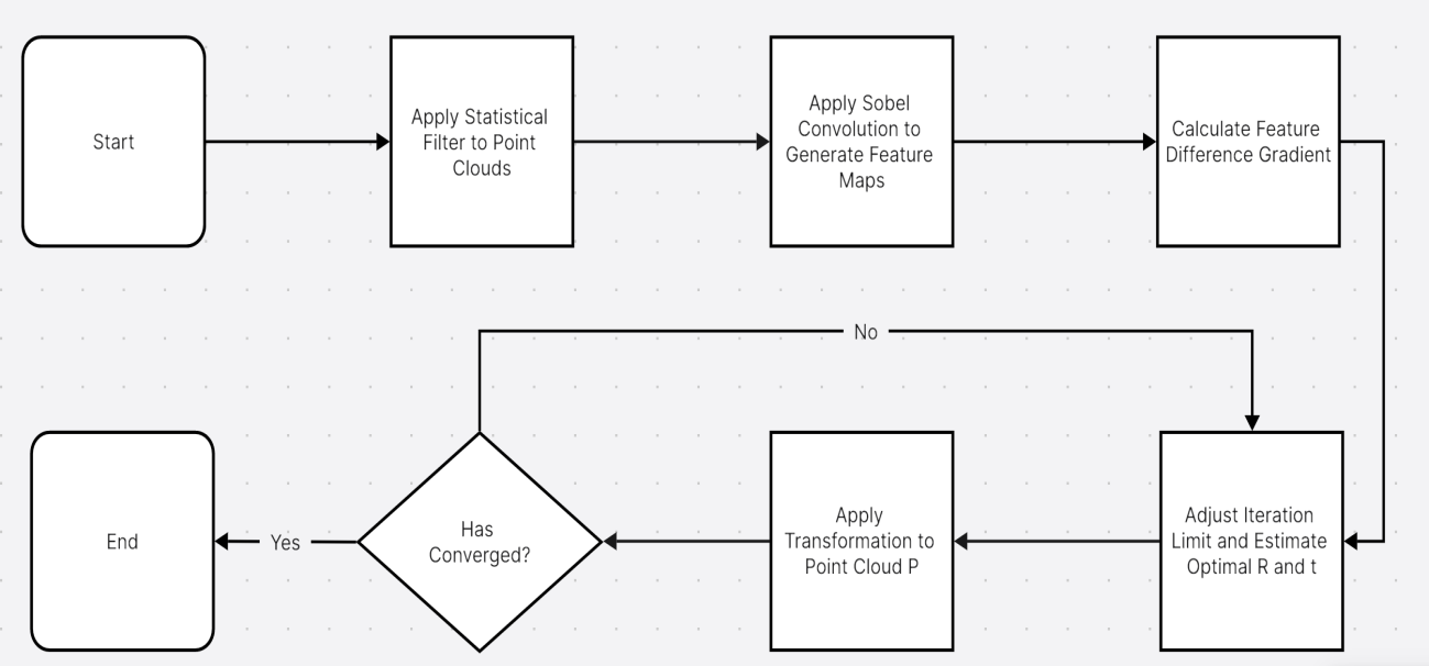
Figure 1. Flowchart of the Improved ICP Algorithm Process

Figure 1 shows the key steps of the improved Iterative Closest Point (ICP) algorithm, which uses a flexible and adaptive way to align point clouds. By using local feature differences, it is possible to reduce the root mean square error (RMSE) compared with the standard ICP algorithm. Subsequent chapters will discuss the results of this method in detail, including RMSE value and iteration times.

4. Experiment and Analysis

This section will introduce the following contents in turn: Section 4.1: Detailed description and selection of the data set used in the experiment. Section 4.2 and 4.3: The results of standard ICP algorithm and improved ICP algorithm are shown respectively. Section 4.4: The robustness of the proposed algorithm is discussed through detailed experiments based on the specified frame rate interval for all frames of data sets A and B (as described in Section 4.1).

4.1. Experimental Dataset Description

To evaluate the performance of the original and improved iterative nearest point algorithm, in this section, we use two data sets (city data sets A and B) from KITTI visual benchmark suite to conduct a series of simulations. These datasets have been selected to simulate environment of varying complexity, providing a comprehensive testbed for evaluating the robustness and accuracy of the algorithms under study.

Table 1. Summary of Datasets A and B

Table 1 shows the key differences in the environmental conditions and registration parameters between the two scenarios.

Parameter Explanations:

Scene: The environmental conditions or background reflected by each data set. Scenario A is a relatively simple urban environment, while scenario B is more complex and contains moving vehicles.

Dataset Name: The specific name of the dataset in KITTI Visual Reference Kit.

Label: Object categories marked in the dataset, which show the existence of dynamic elements, such as cars and pedestrians, thus increasing the complexity of the registration process.

Registration Interval: This is the rate at which registration is performed within the dataset. To see how the algorithm behaves responsively, registration is done every four frames for both cases.

Optimization adjustment factor: it is used to optimize the specific scaling factor in ICP algorithm. In Scenario A, the factor is reduced to reduce the impact of dynamic changes, while in Scenario B, it adopts a higher optimization level to cope with the increase of environmental complexity.

4.2. Original ICP Algorithm

In order to establish the benchmark for evaluating the improved ICP algorithm, we first implement the original point-to-plane ICP algorithm with default parameters. This section will elaborate the process in detail and show how the algorithm works on two frames of point cloud data. In sections 4.2 and 4.3, we selected the 16th and 19th frames in Scene B to control the variables.

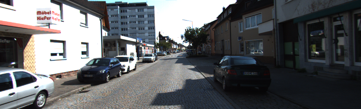
16th frame

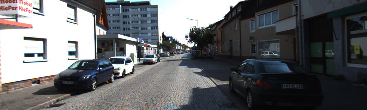
19th frame

Figure 2. Scenario B: Frames 16 & 19 Comparison

Figure 2 shows images of these two frames to show the differences and ensure the consistency of the evaluation.

Firstly, we use the file input/output function of MATLAB to read and process point cloud data from two independent frames, load binary data and extract X, Y and Z coordinates, thus forming point clouds “ptCloud1” and “ptCloud2”. Then, we use the point-to-plane ICP algorithm, which can effectively align smooth surfaces by minimizing the distance from a point in one point cloud to a plane in another point cloud. Using MATLAB’s “pcregistericp” function with its default 30 iterations, the source cloud (ptCloud1) was aligned with the target cloud (ptCloud2). The algorithm minimized the RMSE between the aligned points and the target planes. Given the high density of point cloud data, the visualization is focused on a prominent central section, allowing for a clearer comparison of the differences before and after alignment. Figure 3 shows the visualization of the 3D point clouds.

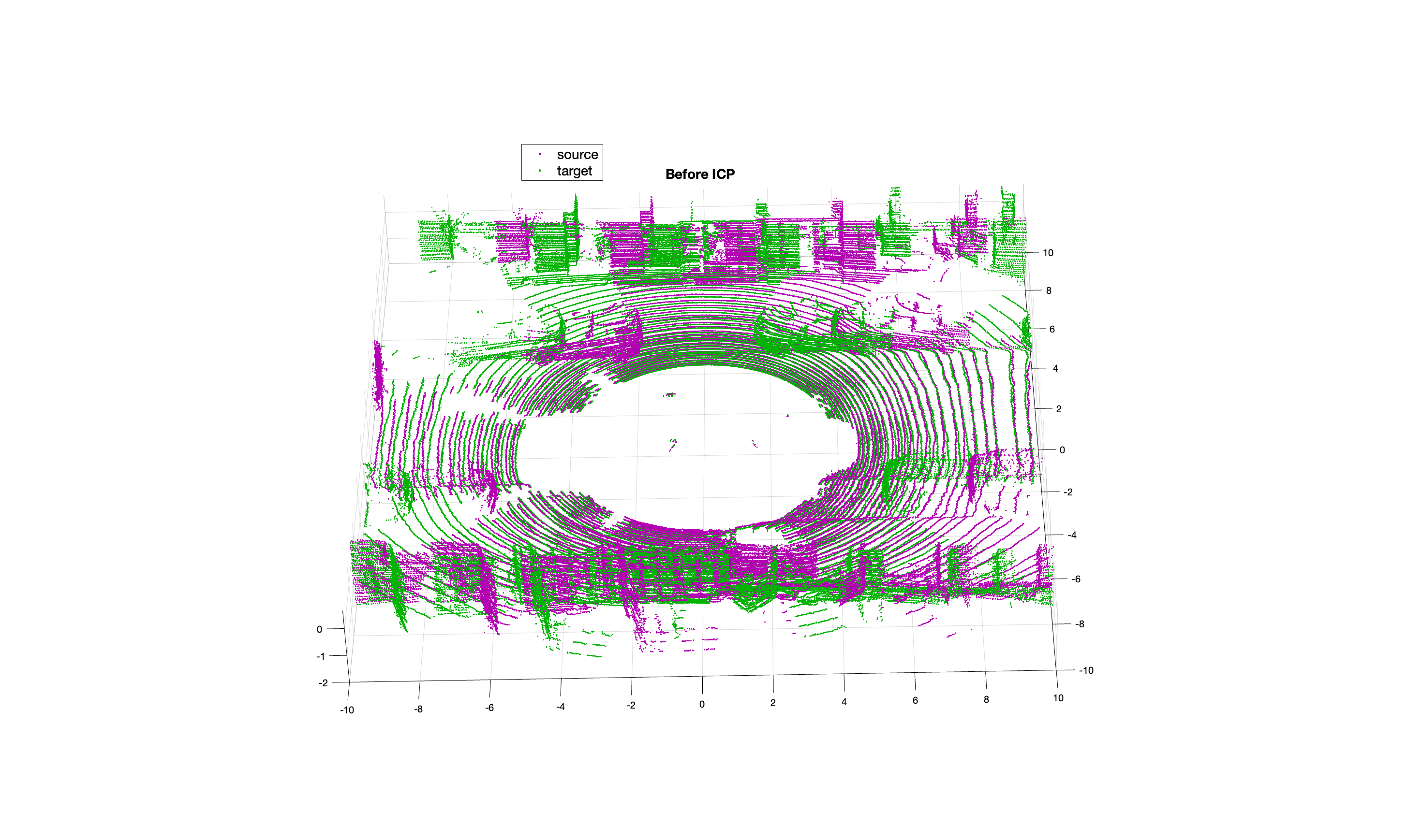
Before Default ICP

After Default ICP

Figure 3. the point clouds before and after applying the ICP algorithm

Using the default point-to-plane ICP algorithm, the RMSE was 0.5578, indicating the algorithm's performance, with lower values representing better alignment. Figure 3 shows some improvement, but the degree of overlap between source and target point clouds remains limited. This highlights the algorithm's limitations in complex environments, where greater accuracy and overlap are needed. Establishing this baseline with the default ICP sets the stage for evaluating the improvements introduced in our enhanced ICP algorithm, discussed in the next section.

4.3. Improved Algorithm Implementation

In this section, we describe in detail the process of the improved ICP algorithm. These steps highlight the core improvements to the standard ICP method, focusing on feature extraction and dynamic iterative tuning.

Step 1: Preprocessing and Outlier Removal

The process begins by loading and preprocessing the point cloud data. Outliers are removed using a statistical filter to improve point cloud quality.

Step 2: Feature Extraction

We then downsample the point clouds using a voxel grid approach to facilitate efficient feature extraction. When processing the point clouds, a voxel grid is utilized in order to down-sample the data of a point cloud. The voxel grid down-sampling refers to partitioning the data of a point cloud into fixed-sized cubes (voxels), which are then reduced to one representative point to help in reducing noise within the data of the point cloud. This is very important when dealing with complex scenes, as this noise, as well as data redundancy, can severely undermine the alignment accuracy. The down-sampling will reduce the number of data represented within the point cloud, hence reducing the computational burden in subsequent processes; this is very significant when a large-scale point cloud is processed. With the aim to extract the features, Sobel convolution kernel is used for edge detection and detecting notable changes in the point cloud.

Step 3: Feature Difference Calculation

We will calculate the difference of extraction features between two point clouds. By summing the square differences, the weight of these differences can be enhanced, and then normalized.

Step 4: Dynamic Iteration Adjustment

The core innovation of the algorithm is that it dynamically adjusts the maximum number of iterations according to the calculated feature differences, which is considered to be very important to optimize the performance of the algorithm [20]. MaxIterationsBase=30 is used as the default iteration number to ensure the initial convergence of the algorithm in a simpler scenario. Dynamic adjustment verifies the research results of Huang and Lee [20], and they emphasize the importance of dynamic iteration in improving the efficiency and accuracy of the algorithm.

We multiply the logarithmic adjustment factor by 100 and add it to the basic iteration times, and increase the iteration times in complex scenes according to the size of feature differences, so that the algorithm can capture the corresponding relationship between complex geometric structures more effectively. In order to avoid over-fitting or waste of computing resources caused by too many iterations, even in complex scenes, the execution time of the algorithm is kept within the controllable range, and we set the maximum number of iterations. We use dynamically adjusted iteration times for ICP registration to achieve better registration effect.

Step 5: Visualization of the Registration Process

The results of the visual registration process can be obtained for comparison between the default ICP algorithm and the improved one, with dynamic iterative adjustment. Such visual comparisons can effectively evaluate the effectiveness of the improved ICP algorithm to show how it aligns point clouds better through dynamic adjustment and also attains higher registration accuracy as compared to the default ICP algorithm.

a. after default ICP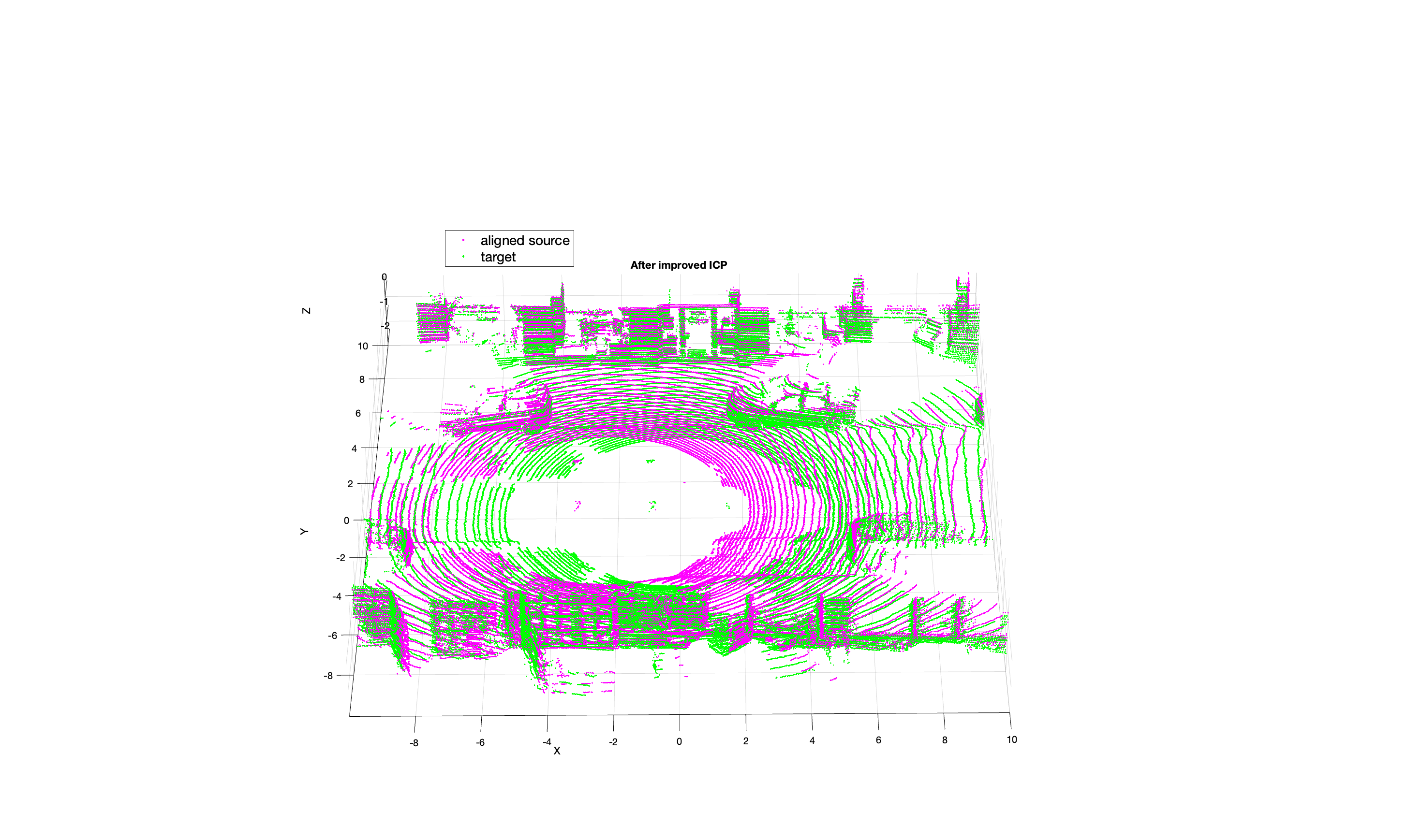b. ICP after improvement

Figure 4. Comparison of point cloud registration results

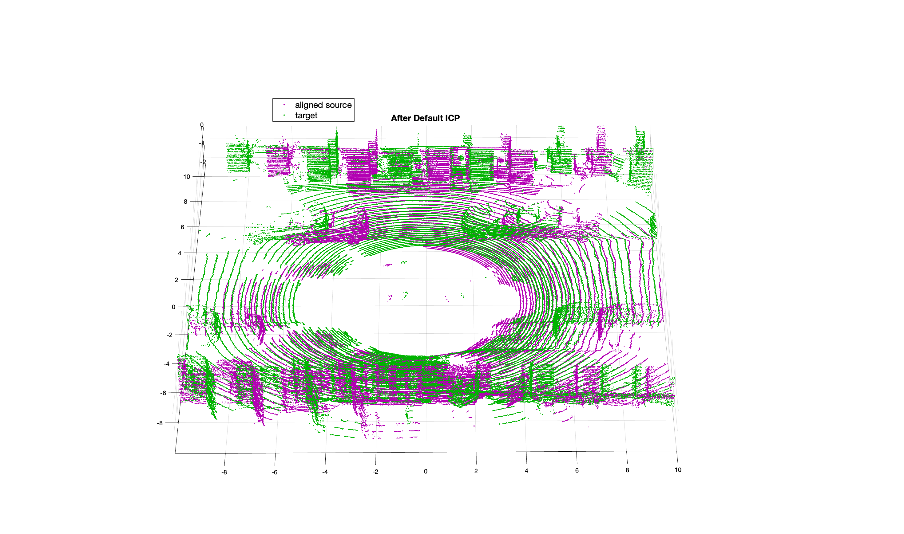
Figure 4 shows a comparison of point cloud registration results using default ICP and improved ICP. The purple points are the source or non-registered point cloud and are given as input to the program, while the green points are the target or registered point cloud, acting as a reference when the point clouds are transformed. Initially, a large disparity could be noted in the displacement or rotation between the purple (source) and green (target) points. As the registration progresses, a successful alignment is indicated by an increased overlap between the purple and green points. The greater the overlap, the higher the registration accuracy achieved.

The improved algorithm has a significantly higher overlap rate, especially when dealing with complex objects such as vehicles, buildings, and cobblestone surfaces, which shows that it is excellent at accurately identifying and aligning these detailed features.

In the final experiment, we dynamically adjust the improved ICP algorithm, and the maximum number of iterations is 131, with a mean square error of 0. 4064. In contrast, the traditional ICP method only has 30 fixed iterations at most, and the RMSE is 0.5578, which shows that the accuracy of the improved algorithm has been significantly improved. Through adaptive iterations, the algorithm can deal with the change of point cloud more flexibly and realize more accurate registration. This improvement highlights the effectiveness of feature-based adjustment in optimizing registration process.

Step 6: Validation of Convergence and Overfitting Avoidance

We conducted additional experiments to evaluate the root mean square error in different iterations to test the robustness and optimality of the algorithm in the iteration, and to ensure that the number of iterations (131) selected in the dynamic adjustment algorithm will not lead to over-fitting or insufficient convergence.

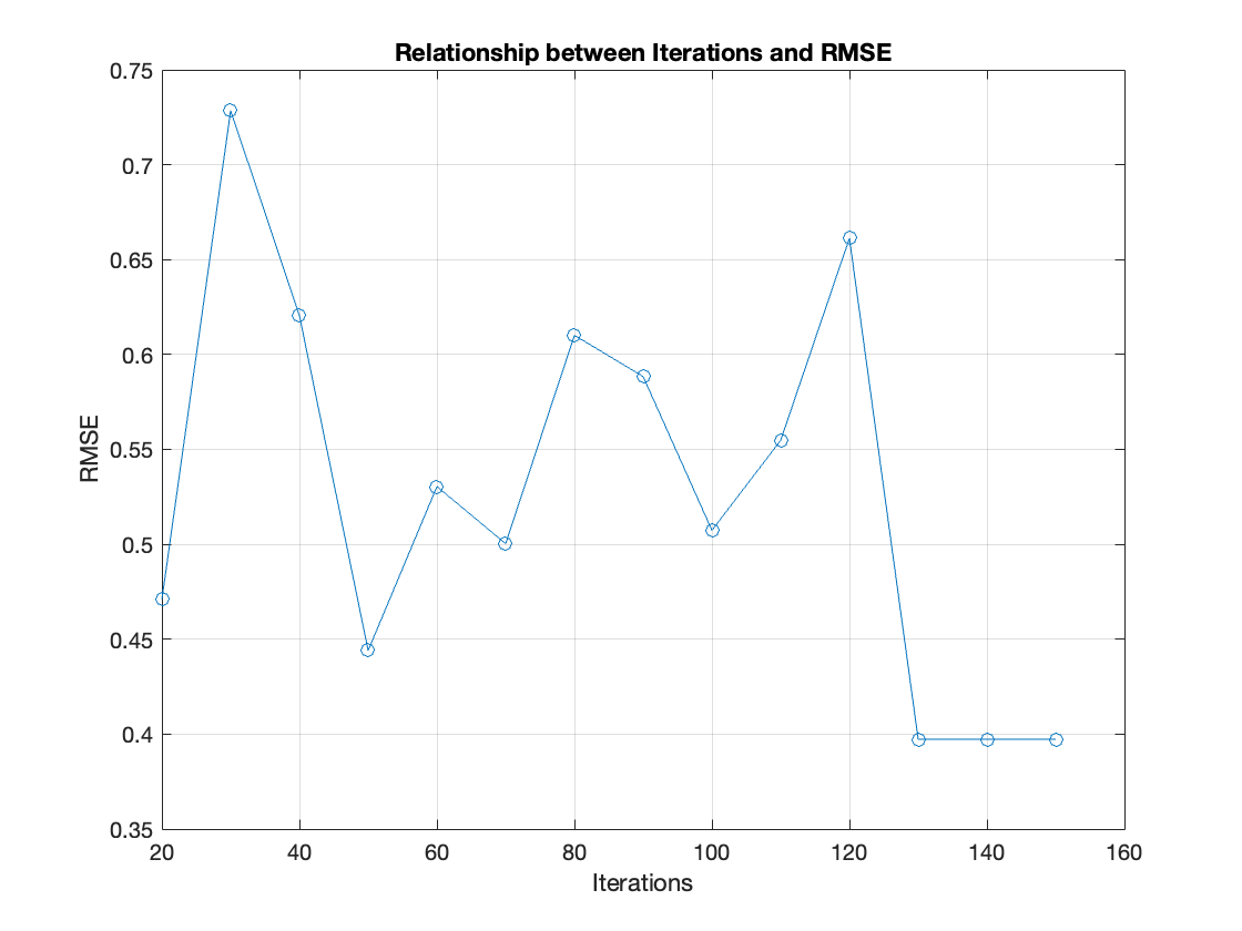
Figure 5. Relationship between Iterations and RMSE

Figure 5 is a plot of the relationship between RMSE and the number of iterations. The RMSE in this graph decreases first with the number of iterations and then stabilizes after some. That means the chosen number of iterations of 131 is an optimal one for this alignment task as it effectively avoids overfitting and ensures sufficient.

4.4. Data Analysis

Analyzing the experimental data of scenes A and B shows the influence of the improved ICP algorithm compared with the original ICP algorithm. The results are summarized as follows according to Table 2

Table 2. Comparing the original ICP algorithm in Scenes A and B

In Scenario A, the average root mean square error of the original ICP algorithm is 0.5285 mm due to less environmental challenges. After the application of the optimization algorithm, this value is reduced to 0.4892 mm, showing an improvement of 7.4%. This modest improvement shows that the algorithm can still improve the alignment accuracy in simple scenes and achieve accurate registration with low computational overhead.

In more complex scenario B, the RMSE of the original ICP algorithm is 0.5191 mm. After the application of the optimized algorithm, the numerical value is reduced to 0.4212 mm, an increase of 18.9%, which shows the strong stability of the algorithm in complex urban environment.

Because the algorithm performs better in dealing with the variability and complexity of the environment, scene B is significantly improved, including dense point clouds, more occlusion and higher noise level, which is consistent with our research assumptions, indicating that the optimized ICP algorithm is particularly effective in complex environments, and its ability to dynamically adjust and optimize the registration process is more prominent in such situations.

Because the improved ICP algorithm has dynamic characteristics, we decided not to average the number of iterations in these experiments. The algorithm automatically adjusts the number of iterations according to the feature differences between point clouds, so the number of iterations will change according to the complexity of the scene and the alignment requirements. Averaging the number of iterations in different experiments will cover up these dynamic adjustments, thus reducing the clarity of analysis. We should focus on the adaptability of the algorithm, not the number of static iterations. In addition, the effectiveness of the improved ICP algorithm is better reflected by the root mean square error value, which directly reflects the alignment quality.

These scenarios show the adaptability and efficiency of the algorithm under different complexity. In Scenario B, the performance is significantly improved, which further proves that the optimized ICP algorithm is outstanding in a more challenging environment, so it is very suitable for urban applications with complex and changing environments.

5. Conclusion

Compared with the traditional method, the optimized ICP algorithm shows obvious progress in the simple and complex urban environment, the method dynamically adjusts parameters according to the complexity of the scene, and improves the accuracy of point cloud registration. This makes it more robust in difficult situations. This adaptive algorithm not only reduces the root mean square error (RMSE) of the algorithm, but also improves the performance of the algorithm under various conditions.

This paper has proposed an optimized ICP method for the handling of noisy and complex environments, which may find applications in SLAM methods, autonomous driving, and 3D mapping. Its robustness in these challenging scenarios is of great practical importance. In the following works, the algorithm will be combined with machine learning techniques to increase its adaptability and the accuracy even further. Lastly, the scalability and real-time nature of the evaluated algorithm mean that it will pave the way for new applications in time-sensitive operations and provide key insights into its deployment in autonomous systems and other dynamic environment.

Acknowledgement

We are very grateful to Professor Danijela Cabric for her valuable guidance in the whole project, and we are also grateful to Assistant Professor Zhong Zhiyuan for his support at the beginning of the work. In addition, the open source data provided by KITTI Visual Benchmarking Suite is very important for our research. Finally, thank the whole team for their hard work and good cooperation.

References

[1]. Durrant-Whyte, H., & Bailey, T. (2006). Simultaneous localization and mapping: part I. IEEE robotics & automation magazine, 13(2), 99-110.
[2]. Mur-Artal, R., Montiel, J. M. M., & Tardos, J. D. (2015). ORB-SLAM: A versatile and accurate monocular SLAM system. IEEE Transactions on Robotics, 31(5), 1147-1163.
[3]. Engel, J., Sturm, J., & Cremers, D. (2012). Camera-based navigation of a low-cost quadrocopter. In 2012 IEEE/RSJ International Conference on Intelligent Robots and Systems (pp. 2815-2821). IEEE.
[4]. Engel, J., Schöps, T., & Cremers, D. (2014). LSD-SLAM: Large-scale direct monocular SLAM. In European conference on computer vision (pp. 834-849). Springer, Cham.
[5]. Biber, P., & Straßer, W. (2003). The normal distributions transform: A new approach to laser scan matching. In Proceedings of the IEEE/RSJ International Conference on Intelligent Robots and Systems (pp. 2743-2748). IEEE.
[6]. Mur-Artal, R., & Tardos, J. D. (2017). ORB-SLAM2: An open-source SLAM system for monocular, stereo, and RGB-D cameras. IEEE Transactions on Robotics, 33(5), 1255-1262.
[7]. Williams, B., Klein, G., & Reid, I. (2007). Real-time SLAM relocalisation. In 2007 IEEE 11th International Conference on Computer Vision (pp. 1-8). IEEE.
[8]. Besl, P. J., & McKay, N. D. (1992). A method for registration of 3-D shapes. IEEE Transactions on pattern analysis and machine intelligence, 14(2), 239-256.
[9]. Rusinkiewicz, S., & Levoy, M. (2001). Efficient variants of the ICP algorithm. In Proceedings Third International Conference on 3-D Digital Imaging and Modeling (pp. 145-152). IEEE.
[10]. Seitz, S. M., & Dyer, C. R. (1999). Photorealistic scene reconstruction by voxel coloring. International Journal of Computer Vision, 35(2), 151-173.
[11]. Chen, Y., & Medioni, G. (1991). Object modeling by registration of multiple range images. Image and vision computing, 10(3), 145-155.
[12]. Sara, R. (2005). The class of stable matchings for ICP-based registration. In Proceedings of the IEEE Computer Society Conference on Computer Vision and Pattern Recognition (CVPR) (Vol. 1, pp. 128-133). IEEE.
[13]. Chen, A., & Zhuang, J. (2022). An Improved ICP Algorithm for 3D Point Cloud Registration. In 2022 3rd International Conference on Pattern Recognition and Machine Learning.
[14]. Zhang, Z. (2010). A Statistical Method for ICP Algorithm. In Journal of Computer Vision.
[15]. Bouaziz, S. (2016). Sparse-ICP: An Algorithm for Robust Point Cloud Registration. In Proceedings of the IEEE Conference on Computer Vision and Pattern Recognition.
[16]. Zhang, Y. (2018). FRICP: Fast and Robust ICP Algorithm. In International Journal of Robotics Research.
[17]. BO-ICP (2022). Initialization of Iterative Closest Point Based on Bayesian Optimization. In IEEE Transactions on Robotics.
[18]. Rusinkiewicz, S., & Levoy, M. Efficient Variants of the ICP Algorithm. Stanford University.
[19]. Gonzalez, R. C., & Woods, RichardE. (2014). Digital Image Processing 3rd Edition.
[20]. Mitra, N. J., Gelfand, N., Pottmann, H., & Guibas, L. (2004). Registration of point cloud data from a geometric optimization perspective. Proceedings of the 2004 Eurographics/ACM SIGGRAPH Symposium on Geometry Processing. Presented at the SGP04: Symposium on Geometry Processing, Nice France. https://doi.org/10.1145/1057432.1057435
Cite this article
Zhu,T.;Mao,Y.;Zhang,J. (2025). Adaptive Iterative Control Optimization ICP Algorithm for Robust Point Cloud Registration in Urban Environments. Applied and Computational Engineering,132,83-94.
Data availability
The datasets used and/or analyzed during the current study will be available from the authors upon reasonable request.
Disclaimer/Publisher's Note
The statements, opinions and data contained in all publications are solely those of the individual author(s) and contributor(s) and not of EWA Publishing and/or the editor(s). EWA Publishing and/or the editor(s) disclaim responsibility for any injury to people or property resulting from any ideas, methods, instructions or products referred to in the content.
About volume
Volume title: Proceedings of the 2nd International Conference on Machine Learning and Automation
© 2024 by the author(s). Licensee EWA Publishing, Oxford, UK. This article is an open access article distributed under the terms and
conditions of the Creative Commons Attribution (CC BY) license. Authors who
publish this series agree to the following terms:
1. Authors retain copyright and grant the series right of first publication with the work simultaneously licensed under a Creative Commons
Attribution License that allows others to share the work with an acknowledgment of the work's authorship and initial publication in this
series.
2. Authors are able to enter into separate, additional contractual arrangements for the non-exclusive distribution of the series's published
version of the work (e.g., post it to an institutional repository or publish it in a book), with an acknowledgment of its initial
publication in this series.
3. Authors are permitted and encouraged to post their work online (e.g., in institutional repositories or on their website) prior to and
during the submission process, as it can lead to productive exchanges, as well as earlier and greater citation of published work (See
Open access policy for details).