1. Introduction

Horse racing is a sport involving two or more professionally trained jockeys competing on horses that has amassed a large audience worldwide, where the performance of the horses is influenced by a variety of factors. One factor, the condition of the racing surface, known as the going, is crucial. Track going is classified in a range from firm to heavy, with firm signifying that the track is very dry and in great racing condition and heavy meaning that the track is very wet and difficult to run on. This variability can significantly impact the outcome of races, affecting both the horses' performance and the strategies employed by trainers and jockeys. Accurate reporting of track conditions is thus essential for ensuring fair competition.

Despite the importance of track going in determining race finishing times and outcomes, there are concerns regarding the accuracy and consistency of these reports. In this context, even minor inaccuracies in the reported track conditions can have consequences. Trainers may misjudge the suitability of the track for their horses, bettors may place wagers based on incorrect information, and the overall integrity of the sport may be questioned. This study addresses these concerns by examining the reasonableness of reported track goings in accordance with other race conditions.

The objective of this research is to model horse racing finishing times to confirm the validity of reported track goings. By analyzing a comprehensive dataset from three racecourses—Catterick, Chester, and Newmarket—we aim to uncover patterns and discrepancies that may point towards inaccuracies in the reported track conditions. These courses all share dirt surfaces that are susceptible to changes in going and we only explored the flat races ran with no hurdles.

This holds notable implications for the horse racing industry. By improving the transparency and reliability of track condition reports, bettors and stakeholders can make fully informed moves, leading to fairer competition and increased trust in the sport's integrity. Accurate reporting of track goings can mitigate financial losses for bettors and ensure that trainers and jockeys have the reliable information they need to prepare their horses effectively. Furthermore, this study contributes to the broader field of sports analytics by demonstrating how data-driven approaches can be applied to verify and improve the accuracy of reported information.

2. Literature Review

Much work has been done in previous years to analyze horse racing. However, most studies instead focus on the aspect of horse racing that is most applicable to betting, which is the winning horse. In our investigation, we found no prior work on predicting or correcting the suspicion of incorrectly reported course conditions. Since even more factors affect the outcome of which horse will win, researchers have explored a variety of algorithms to improve racing predictions. This review details the different approaches and algorithms used by different researchers to create prediction models, focusing on Artificial Neural Networks (ANN), Support Vector Regression (SVR), and other techniques.

2.1. Artificial Neural Networks (ANN)

Artificial Neural Networks are frequently used in horse racing predictions because of their usefulness in modeling complex relationships between input variables and outcomes. This method involves creating a network of nodes (neurons) that process input data through layers, ultimately predicting the outcome of the race.

Williams and Li [1] conducted their research on predicting the outcomes of horse races in Jamaica using ANN. 143 races between January and June 2007, with race distances ranging from 1 to 3 kilometers was used as data. They fed variables, including horse, jockey, past race positions, track distance, and finishing times, into their ANN model. To optimize the model's performance, they compared four different learning algorithms, dividing the data into 80% for training and 20% for testing. This resulted in a 70% accuracy for the ANN model. Similarly, Davoodi and Khanteymoori [2] used an ANN to predict horse racing outcomes at a single race track in New York. Their data originated from 100 races starting in January 2010,using horse weight, race type, trainer, jockey, the number of horses in a race, track distance, and weather conditions as input variables. They experimented with five different supervised learning algorithms, including Gradient Descent Backpropagation (BP), Gradient Descent BP with momentum, Quasi-Newton BFGS, Levenberg-Marquardt, and Conjugate Gradient Descent. The study found that while the BP and BP with momentum algorithms were more accurate, the Levenberg-Marquardt algorithm was the fastest. The algorithms achieved an average accuracy of about 77%.

Besides horse racing in sports betting, ANN has also been applied to other topics as seen in Baulch's research on predicting winners in rugby league and basketball games [3] and also for predicting NFL results [4]. In his research, Baulch used Backpropagation and Conjugate Gradient methods that relied on past team performance data such as win-loss records and average scores per game. The accuracy levels for rugby ranged from 55% to 58.2%, whereas those for basketball were between 49% and 59%. These findings suggest that the ANN has been a useful tool for sports predictions where its accuracy is relative to the quantity as well as quality of input data. An improvement in this area has been explored by predicting link directions to account for incomplete real-world information [5,6]. Guo and Yang tested this method of link predicted with success using recursion on nodes of different ranks on real-world data from various sources, including the neural networks of C. Elegans and Facebook posts from New Orleans, Florida.

2.2. Support Vector Regression (SVR) and Other Methods

Support Vector Regression (SVR) is another technique used to predict race outcomes. It is an ML algorithm which typically involves finding a hyperplane that best fits data, making it possible to predict continuous values such as finishing times of horses in races.

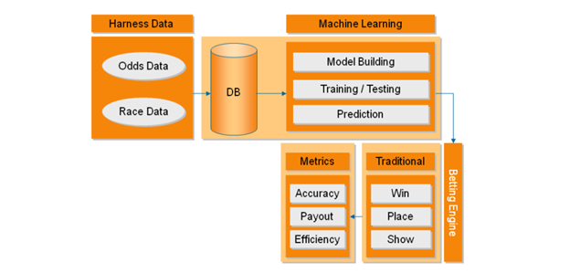
Figure 1. The S&C Racing System [4]

Robert P. Schumaker[7] applied SVR to predict horse rankings in upcoming races. His model, The S&C Racing System, had an amalgamation of several components: a data module, machine learning algorithms, a betting engine, and evaluation metrics (Fig.1). Schumaker's model, like the ones before it, took into account many features from previous races such as fastest times, win percentage, place percentage and average finishing positions. He did not only focus on the prediction accuracy but also in the sense of applying different betting strategies for maximum payout optimization — such as Win/Place/Show. The S&C Racing System found this happy medium where the payout was maximized without losing too much on accuracy.

In an extension of Schumaker's work, Schumaker and Johnson[8] developed a similar SVR approach for greyhound races. With data from over 1,900 races across 31 different dog tracks, they developed a model called the AZGreyhound System. It included several betting engines, including more complex wagers like Exacta, Trifecta, and Superfecta. These bets required predicting the exact placement of multiple dogs, increasing the complexity of the prediction task. The system was evaluated for accuracy, payout, and efficiency, with findings indicating that while higher accuracy often led to lower payouts, and vice versa, the system was effective in managing this trade-off.

Another study using SVR for horse racing predictions involved 20 different features, each assigned a value of -1, 0, or 1 [9]. The model was trained on data from December 2016 to February 2017 and tested in March 2017. Results were then compared to a baseline known as the morning line, a pre-race estimate of betting odds provided by a track handicapper. The SVR model outperformed the baseline, achieving a winning percentage of 28% compared to the baseline's 26%, and had higher overall accuracy in predicting horses that finished in the top three positions. This comparison highlights the superiority of machine learning models like SVR over traditional handicapping methods in predicting race outcomes.

In addition to ANN and SVR, researchers have explored other methodologies and hybrid models to predict racing outcomes, often combining multiple algorithms or incorporating domain-specific features to enhance predictive performance. An illustrative example is the work done by Bhooshan et al. [10], who studied network analysis for predicting outcomes in Major League Baseball (MLB) and the National Football League (NFL). They developed directed graphs representing win-loss relationships between teams, with the edges weighted based on the number of victories or losses between teams. Their ranking algorithm allowed them to order teams based on their overall performance, categorizing them into leaders and followers. They also employed logistic regression to predict game outcomes, comparing their results with traditional expert rankings. The network analysis approach proved more objective and accurate, particularly in the NFL, where it accounted for the entire season's performance rather than just recent games.

A study by Hsinchun Chen and colleagues [11] used ANN and the ID3 algorithm to predict greyhound racing outcomes. They initially inputted 50 different variables but later filtered out less significant ones to improve the neural network's performance. The ANN model achieved better payouts, despite lower accuracy compared to human experts, indicating that it was more effective in identifying profitable bets. The researchers reached 34% accuracy with the ID3 algorithm and a payout of $69.20, while the ANN achieved 20% accuracy but a higher payout of $124.80. This study underscores the importance of balancing accuracy and financial return in predictive modeling.

3. Data Preprocessing

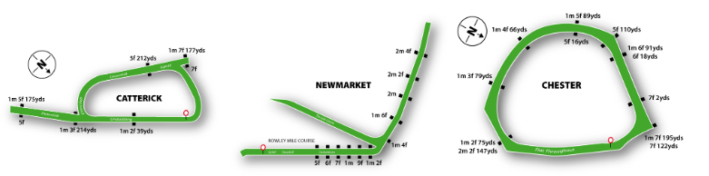
(a) Catterick Course (b) Newmarket Course (c) Chester Course

Figure 2. Course layout of the three utilized tacetracks [12]

The maps above show the layouts of each of the courses in the data and their valid racing distances. We noticed that many of the distances, especially in Chester and Newmarket, fell between even furlongs (1 furlong = 220 yds). In the data, however, all races had distance values in yards that would correspond to integer furlongs. This led to the suspicion that the distances had been previously rounded to the nearest furlong to avoid the variability in race distances often reported by racetracks.

Table 1. Every relevant variable available in the utilized dataset, along with a description, excluding extraneous logical variables for race classification

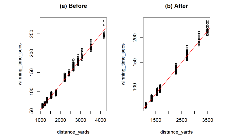
(a) Before (b) After

Figure 3. Linear Models of Winning Time Compared to Distance in Chester Racecourse Before(a) and After(b) Data Cleaning.

Specifically in the data for Chester, there were a group of races with distances of 8 furlongs but there isn't an official 8-furlong length at Chester (Figure 3a). We theorize that all the 7 furlong and 122-yard races been rounded to 8 furlongs and caused a group of races that were way faster than expected for 8 furlongs. This issue was also prevalent in Catterick, where many distances were different than the official reported distances and may have been rounded to the nearest furlong, sometimes changing the actual distance by over 50 yards. Undoing the suspected rounding of the distances for each course to their officially sanctioned distances helped to produce more accurate predictions.

Additionally, in our data, only a few races were conducted at certain distances, especially longer ones greater than 12 furlongs. With ~4000 races in total, we removed the data at these underrepresented distances with under 100 races to reduce noise and ensure that our predictions would be accurate and based on an ample amount of data. Based on the same concept, we also removed a few races with extreme classes like 1 or 7 from the courses that only a few races at those classes over the 10-year period. These adjustments helped the data as a whole slightly but improved course specific accuracy substantially. In the case of Chester, these adjustments lowered the residual standard error of a linear model on winning time to distance from 5.4s to 3.7s and increased the R-Squared value from 0.985 to 0.991 (Figure 3b).

4. Methods

4.1. Dataset Exploration

With a variety of variables tracking a race's circumstances, it is necessary to determine their individual impacts on a prediction of the winning time (Table 1). Without this sorting, the additional time complexity of considering every variable would make any meaningful predictions impossible to compute. Firstly, the most intuitive and important of the variables that can affect the winning time is the length of the race, or “distance_yards” in the data.

Across the 3 courses, there are only 15 distinct distances in which races were conducted, which makes it possible to group races together by distance in order to study the impact of the other variables upon their times. This is necessary because if we were to study all distances at the same time, it would be generally useless as there would be gaps in the winning time data caused by the distances.

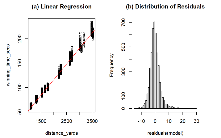
(a) Linear Regression (b) Distribution of Residuals

Figure 4. Linear Regression of Winning Time to Race Distance for All Courses (a) and a Histogram of the Residuals (b)

A linear regression of just distance against time with no other variables is very strong already and gives an R-Squared value of 0.9901 (Figure 4). The residuals of the model are also skewed slightly to the right (Figure 4b). This is caused by the other aforementioned track conditions (Table 1). To study the effect of other variables on winning time independent of distance, we plotted the variables against winning time for every distance and looked at them as a whole. The most standout variables were going and class.

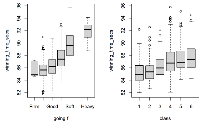
(a) Ground Condition (b) Horse Quality

Figure 5. Boxplots between Winning Time and Going (a) and Class (b) across all courses at a distance of 1540 yards

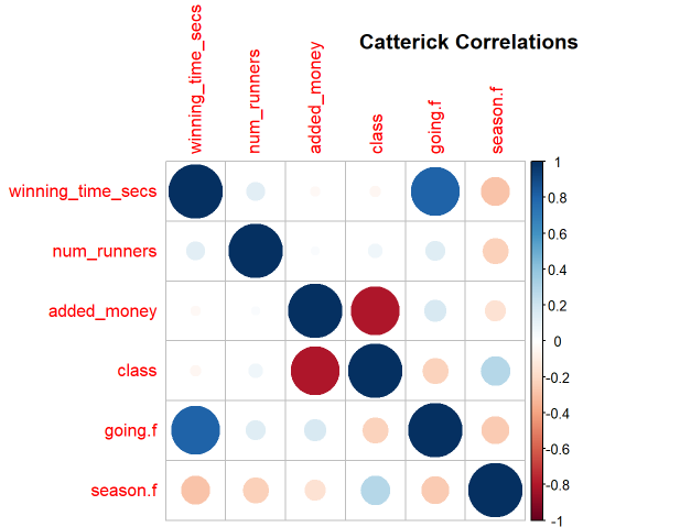
Figure 6. Correlation Plot of Relevant Variables in the Chester Racecourse, with Circle Size and Color Corresponding with Correlation Strength

The relationship between going and winning time is very logical as horses are expected to be slowed down by muddy soil, which is why we see such a strong influence. As the goings get worse, the winning times become slower and this trend is not linear ( Figure 5a). Class too, is logically justified as races with better horses are expected to finish faster. This is why we see a slight trend downwards in winning time as the class decreases, signifying better jockeys and horses (Figure 5b). In the case of course specific correlations across all relevant variables, a strong correlation between added_money and class is evident across the courses (Figure 6). This makes sense as more prestigious races will attract higher bets Figure 5 shows many weaker correlations as well. For example, the season the race was conducted in seems to have some effect on the times. However, they are largely irrelevant. In conclusion, we are left with these strong variables to consider:

(1) course: multiple differences between the three courses

(2) date: will be used in final daily analysis of going

(3) winning_time_secs: our response/predicted variable

(4) distance_yards: a longer distance leads to higher winning time

(5) class: better horses usually run better

(6) going: ground quality heavily influences speed

4.2. Linear Model

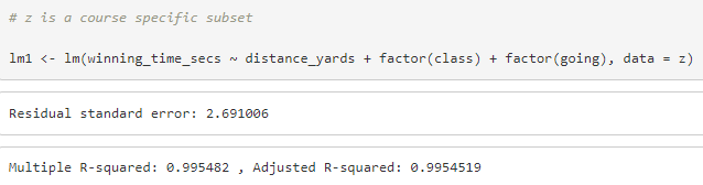
Figure 7. Linear regression model and the outputs

To obtain expected winning times for each of the different goings, we construct a linear model that takes the most important variables into account. The code for this model in R can be seen above. Using this, we set distance in yards as the x- axis, and winning time in seconds as y-axis. The other variables like class and going are treated categorically because going is not numerical and class does not affect the winning time linearly in all courses. We are also not considering and interactions between the variables. This means that in this version of the model, class and going do not affect the slope of the regression, making all the regression lines for each going parallel. However, after noticing that the longer distances are seeing higher variability, we made some changes.

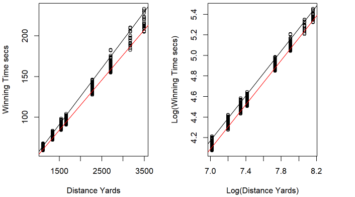
(a) Original Scale (b) Log-Transformed Scale

Figure 8. Plots of winning time to distance in yards with lines demonstrating changes in variance as distance increases before (a) and after (b) a log transformation

Figure 9. Discrete R Code for log transformed linear regression model

Since one of the prerequisites to making a linear model is homoscedasticity, or consistent variance, and our original model's variance increased significantly over time, it was invalid (Figure 8a). To correct this, we took a log of both sides to eliminate the heteroscedasticity and achieve a more appropriate model (Figure 8b). In this version of the model, we are also considering the interaction between the different goings and the distance of the races so that the slope of each regression line for the goings can be different. Since the goings affect the distances differently, specifically affecting the longer distances more, this also helped to build a more comprehensive model. Going forward, all calculations were made with the corrected 2nd linear model.

To achieve the goal of determining whether reported goings are reasonable given specific race circumstances, we employ a prediction interval to find the upper and lower bounds of winning time that are reasonable for that race given a going. We do this using the “predict” function in R 4.4.1 [13] that calculates the bounds using the following equation [14], where y-hat represents the predicted winning time, the t value corresponds with the value needed for a 95% confidence, and the expression with the square root is the residual standard error of the prediction:

\( {\hat{y}_{new}}±{t_{\frac{α}{2},n-p-1}}∙\sqrt[]{{\hat{σ}^{2}}(1+x_{new}^{T}{({X^{T}}X)^{-1}}{x_{textnew}})} \)

By iterating through every going that has appeared in a course and calculating a prediction interval for each of them in a specific race, we can then see if the actual winning time of that race falls within these intervals, leaving us with the goings that could reasonably explain the actual winning time. Additionally, during this process, we store the predicted time that is closest to the actual time and log the going that generated the prediction for that time as “most likely.” This may be very important information for the decision making of stakeholders if multiple races in a day have a differing “most likely” going than than the reported one.

4.3. Check the model

As we are using linear regression to estimate the winning time, it is necessary to check whether our model follows the Gauss-Markov assumptions. Here we will use Newmarket to demonstrate our model.

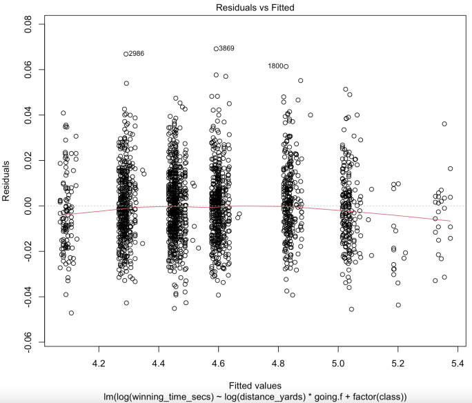
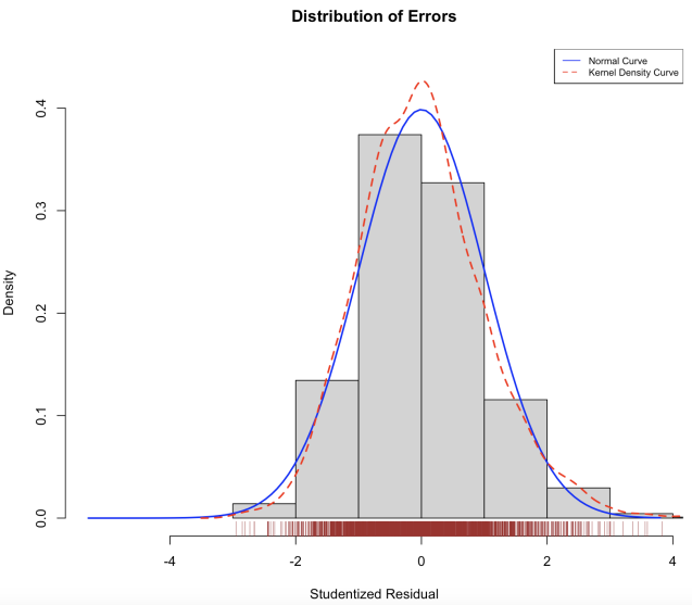
(a) Residuals vs. Fitted Plot (b) Error Distribution Plot

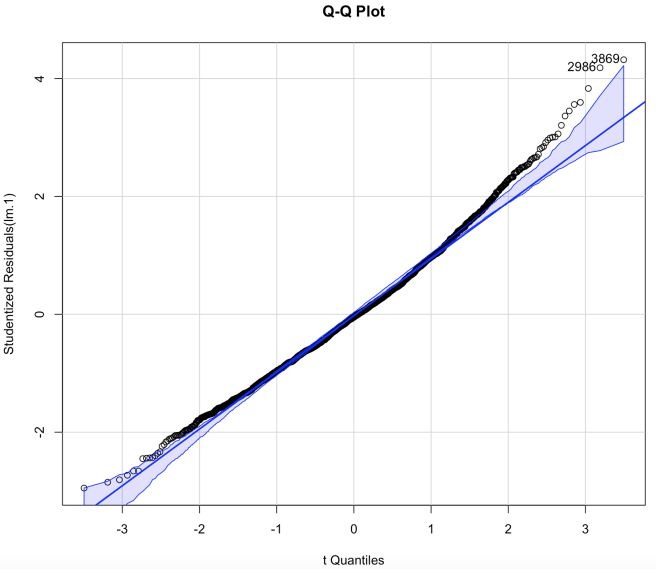
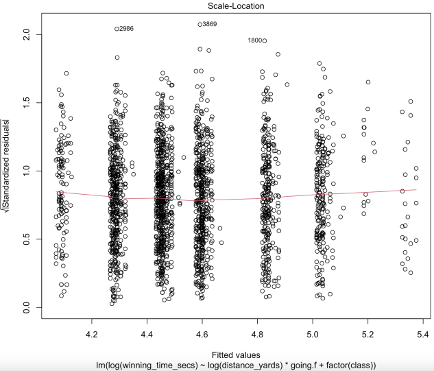
(c) Q-Q Plot (d) Scale-Location Plot

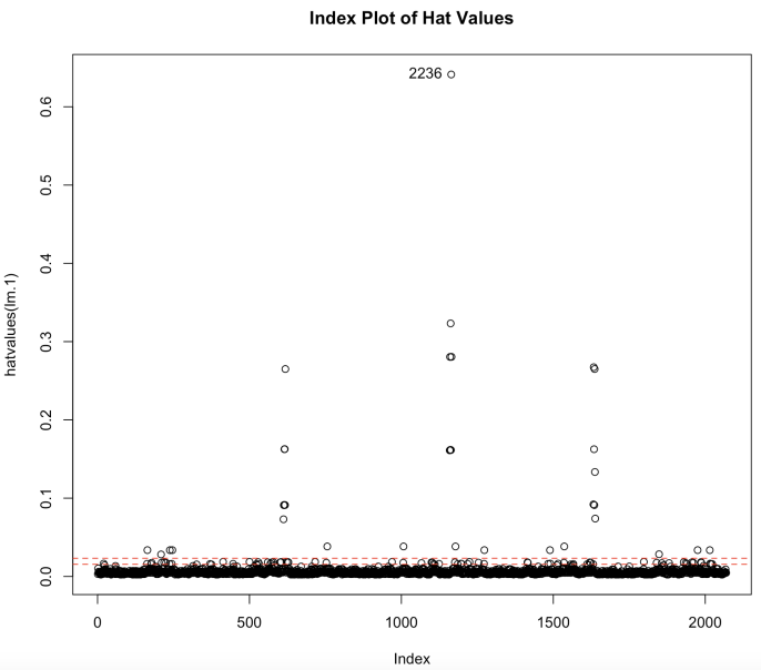
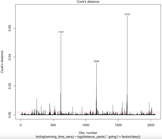
(e) Hat Value Plot (f) Cook’s Distance Plot

Figure 10. Regression Diagnostics Checks for Gauss-Markov Assumptions of Linear Model after Log Transformation and Outliers Detection Specifically in Newmarket Racecourse

Our Residuals vs. Fitted plot (Figure 10a) indicates that there is no systematic relationship between residuals and predicted values, thus the linearity assumption holds. For the assumption of normally distributed errors, the Error Distribution plot (Figure 10b) shows that the errors are roughly normally distributed, the Q-Q plot (Figure 10c) also shows that with 95% confidence, most observations fall around the straight line. Thus, there is no evidence to reject the normality assumption. We’ve previously explained how we are using the log transformation to solve the problem of heteroscedasticity, and the Scale-Location plot (Figure 10d) shows that our transformation is indeed potent. As for the assumption of independence of errors, despite logically there might be a tiny correlation between the goings of races in one day, it is not uncommon to have abrupt change of goings either. Moreover, since distance yards alone explains more than 96% of variance of the data already, it is reasonable to say such correlation in goings is neglectable.

The Q-Q plot (Figure 10c) indicates that #2986 and #3869 have the largest positive residuals. #2236 appears to have prominent hat values in the Hat Value plot (Figure 10e). It also has a high cook’s distance in Cook’s distance plot (Figure 10f), along with #1197 and #3143, indicating they are highly influential to our model.

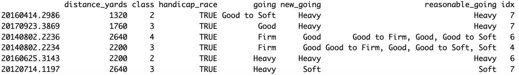
Figure 11. Unusual observations

After closer inspection on these unusual data, we find that the given going is mostly better than the predicted going, indicating that they are running slower than our prediction. Class and distance yards don't seem to explain such a long winning time, but other variables that are not considered in our model do. All these races are handicap races, thus the extra weight may result in the slow speed. Also, these races are mostly the last race of the day, thus we may expect unusual weather or previous races to affect the goings. As there are plenty of data and ruling them out won’t make the model anywhere worse, we decide to remove them from the history data of the Newmarket course.

4.4. Probability Table

To find the probability of each going compared to the actual going based on the actual winning time and the predicted winning times, we used Bayesian Inference [15]. The Bayesian Theorem is a way of making statistical inferences in which the statistician assigns subjective probabilities to the distributions that could generate the data. First, we calculate the likelihood of the actual time given each going by using the probability density function of the normal distribution:

\( P({T_{actual}} | {going_{i}})=\frac{1}{\sqrt[]{2π{σ^{2}}}}exp⁡(-\frac{{({T_{actual}}-T_{predicted}^{(Firm)})^{2}}}{2{σ^{2}}}) \)

Second, we assign the \( P({going_{i}}) \) to be the prior probability of the i-th going condition. As the probability of each going is more correlated with the weather condition today instead of how frequently each going appears in the history, we set that \( P({going_{i}})=\frac{1}{6} \) , as there are 6 goings in total. Finally, based on Bayes’ theorem, we calculated the posterior probabilities of each going given the actual winning time by dividing the product of likelihood and prior probability by the sum of all such products:

\( P({going_{i}} | {T_{actual}})=\frac{P({T_{actual}} | {going_{i}})∙P({going_{i}})}{P({T_{actual}})} \)

By following this approach, we ensure a formal and accurate determination of the posterior probabilities, which are crucial for further analysis and decision-making processes.

5. Results

By looping through all the races after 2018, where there exists enough historical data to make the model function accurately, we make a table of all races after 2018 with additional columns to record our results. The probabilities of each going in one race from column Firm to column Heavy are calculated using the Bayesian theorem. The variable new_going provides the most likely outcome that our model predicts, while the variable reasonable_going stores all the previously defined reasonable outcomes. The column reasonable checks where the given going.f falls in our reasonable going list . We will use the idx column, which stores the index of each race based on the sequence of races on each date, for future studies.

With our model, we check the number of unreasonable goings on each date. We observe that the majority of dates with misjudged goings only contain one or two unreasonable goings, which could potentially be isolated outliers. On the other hand, a date with three or more unreasonable goings may indicate a unique situation that contributes to the date's inaccurate goings.

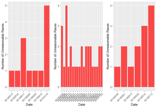
(a) Catterick (b) Newmarket (c) Chester

Figure 12. Histogram of Unreasonable Races by Date for (a) Catterick, (b) Newmarket and (c) Chester

We chose June 30th, 2018 in Newmarket to gain a detailed understanding of why the reported goings on this date are largely unreasonable. The reported going is Good to Firm for all races, but the probability graph suggests that the original going on this date may be Good to Soft. However, from the third race onward, the going starts to deteriorate, suggesting the possibility of heavy rain before the third race.

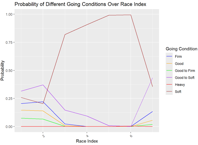
Figure 13. Probability of Different Going Conditions Over Race Index

According to our model, 0.9432314 of the reported goings are reasonable in Catterick. For Newmarket and Chester, this ratio changes to 0.9413989 and 0.9312169, respectively. Given these surprisingly close ratios, one might naturally question whether there are any common factors contributing to the 6 –7% unreasonable goings.

Distance is one possible factor. The longer the races are, the more influence the goings may have on them, potentially leading to more misjudgments. With such hypotheses, we are expecting to see the proportion of unreasonable goings increase with distance increases.

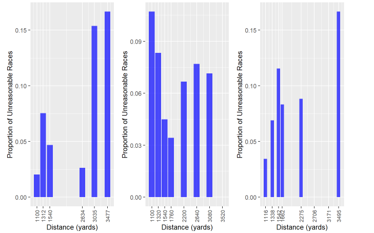
(a) Catterick (b) Newmarket (c) Chester

Figure 14. Proportion of Unreasonable Races by Distance for (a) Catterick, (b) Newmarket and (c) Chester

However, the graph does not support such a hypothesis, particularly for Newmarket, where the trend seems to be the opposite of the other two courses.

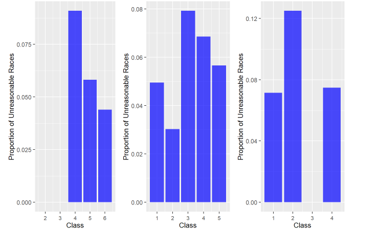
(a) Catterick (b) Newmarket (c) Chester

Figure 15. Proportion of Unreasonable Races by Class for (a) Catterick, (b) Newmarket and (c) Chester

There is no clear relationship between class and unreasonable goings either. Catterick, with fewer class 1 or class 2 races, exhibits a decreasing rate of unreasonable goings with lower class, while the class 1 and class 2 races in Newmarket appear to have fewer unreasonable goings. Chester, on the other hand, having nearly the same amount of class 2 and class 3 races, gets the highest unreasonable rate for class 2 and no unreasonable going for class 3.

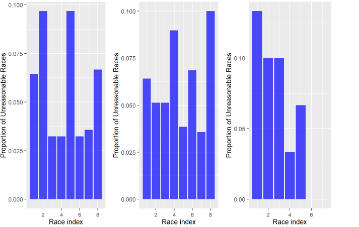
(a) Catterick (b) Newmarket (c) Chester

Figure 16. Proportion of Unreasonable Races by Race Index for (a) Catterick, (b) Newmarket and (c) Chester

We also assign each race an index based on the sequence of races on each day. According to the graph, the first one or two races of the day appear to have more unreasonable goings, whereas the races afterward have fewer. Only a handful of days across all courses will feature more than six races per day, and even though we observe an increase in the rate for the final few races, this could potentially stem from a scarcity of data. However, the higher initial rate may indicate that the results are based on predictions. The impending bad weather may lead the staff to report the going as worse than it actually is.

6. Conclusion and Future Research

In conclusion, by building a linear model that predicts the winning time of each race using all possible goings, we can fairly assess whether the reported goings are reasonable and, if not, identify which goings are more likely to be the actual cases. As anticipated , the majority of reported outcomes are reasonable, although not necessarily precise. For those outcomes that are not reasonable, our probability graphs may also reveal potential factors contributing to the misreporting. Our model allows bettors to get more precise information on the track condition, resulting in better predictions throughout the day as more information about the day's goings is revealed every race.

However, limitations still exist. In our current model, we are using a normal distribution to calculate the upper and lower bounds for the winning times and the probabilities of each going occurring. Since the residuals of our model are not in fact normal, but instead skewed to the right, there may be merit in instead using methods like kernel density estimation to obtain a proper historical distribution instead of using a normal distribution.

Additionally, it is slightly suspicious that the relationship between winning time and distance of the race is linear. We would expect the times to be slightly exponential as horses should not be maintaining a constant speed throughout the races. It is more plausible for them to tire out in longer races and sprint in shorter ones.

Also, our calculations did not take into account some special races that have a significant impact for finish time. Such as the handicap race in which judges assign different weights depending on the competition. Better horses carry heavier weights, which puts them at a disadvantage when competing against slower horses. This question could be solved if we take the weight of the horses into account, we can test whether the weight of each horse is linear with the finishing time. If so, we can add it to our linear model and solve the problem of special races.

The final consideration that we believe to have some merit is in the many extraneous logical variables in the data that were excluded in this paper but were used to classify races. For example, there may be some specific interaction in novice races or amateur races slowing them down due to the inexperience of the jockeys and the horses. There may also be some other factors in seller races and auctions races, where horses are meant to be sold and shown off. In conclusion, there are many ways of creating a stronger and more accurate prediction model, including machine learning algorithms like Random Forest and others like Naive Bayesian and Neural Networks [16]. It would be worthwhile and interesting to see whether those prediction models centered around finding the winning horse could instead be fashioned to detect these inaccuracies in reported course conditions.

Acknowledgements

Mohan Li, Dian Yang, and Tianyu Zhao contributed equally to this work and should be considered co-first authors.

The report was completed under the guidance of Professor John Emerson. His explanation of linear regression models on real-world cases has sparked our interest in horse track analysis. We are thankful for his encouragement and support throughout the research. Additionally, all analysis was done using R 4.4.1 [13] and visualizations utilized the corrplot [17], gt [18], and ggplot2 [19] packages.

References

[1]. Janett Williams and Yan Li, “A case study using neural networks algorithms:horse racing predictions in Jamaica. In International Conference on Artificial Intelligence, Las Vegas, NV, 2008. , ” .
[2]. Ali Reza Khanteymoori Elnaz Davoodi, “Horse racing prediction using artificial neural networks. NN’10/EC’10/FS’10 Proceedings of the 11th WSEAS international conference on nural networks and 11th WSEAS international conference on evolutionary computing and 11th WSEAS international conference on fuzzy systems pages 155-160 . Iasi, Romania June, 2010,
[3]. Michael Baulch, “Using machine learning to predict the results of sporting matches Baulch, M. ”Using Machine Learning to Predict the Results of Sporting Matches”. Department of Computer Science and Electrical Engineering, University of Queensland, 2001. , ”.
[4]. Michael Pardee, “An artificial neural network approach to college football prediction and ranking, ” Technical Paper. Madison, WI: University of Wisconsin, Electrical and Computer Engineering Department, 1999.
[5]. Zimo Yang Guo, Fangjian and Tao Zhou, “Predicting link directions via a recursive subgraph-based ranking Web Sciences Center, University of Electronic Science and Technology of China, Chengdu 611731, PR China, 2013., ”.
[6]. Daniel Hunttenlocher Jon Kleinberg Leskovec, Jure, “Predicting positive and negative links in online social network. Proceedings of the 19th international conference on World wide web, ACM, ” Raleigh, North Carolina, USA April 26 - 30, 2010.
[7]. Robert P. Schumaker, “Using SVM Regression to predict harness races: A one year study of northfield park, ” Computer and Information Science’s Department Cleveland State University, Cleveland, Ohio 44115, USA 2011.
[8]. “Schumaker, Robert P. and Johnson, James W. ”An Investigation of SVM Regression to Predict Longshot Greyhound Races, ” Communications of the IIMA: Vol. 8 : Iss. 2 , Article 7. available at: http://scholarworks.lib.csusb.edu/ciima/vol8/iss2/7, ” 2008.
[9]. Plouffe, Dominic. (2017). “Predicting Horse Racing Results”. Retrieved from https://github.com/dominicplouffe/HorseRacingPrediction
[10]. Wayne Lu Suvrat Bhooshan, Josh King, “Edge direction prediction of sporting tournaments graphs, Stanford University, Final Project, ” 2016.graphs, Stanford University, Final Project, ” 2016.
[11]. Linlin She Siunie Sutjahjo Chris Sommer Daryl Neely Hsinchun Chen, Peter Buntin Rinde, “Expert prediction, symbolic learning, and neural networks: An experiment on greyhound racing, IEEE Intelligent Systems, vol. 9, no. 6, pp. 21-27, ” Journal, Dec 1994.
[12]. At The Races. (2023).Course Guides, At The Races. https://www.attheraces.com/course-guides (Accessed July 24, 2024).
[13]. R Core Team (2021). R: A language and environment for statistical computing. R Foundation for Statistical Computing, Vienna, Austria. URL https://www.R-project.org/.
[14]. Montgomery, D. C., Peck, E. A., & Vining, G. G. (2012). Introduction to Linear Regression Analysis (5th ed.). John Wiley & Sons. (upper lower bound function)
[15]. Statlect. (n.d.). Bayesian inference. Retrieved July 28, 2024, from https://www.statlect.com/fundamentals-of-statistics/Bayesian-inference
[16]. Gulum, Mehmet Akif, “Horse racing prediction using graph-based features.” (2018). Electronic Theses and Dissertations. Paper 2953.
[17]. Taiyun Wei and Viliam Simko (2021). R package ‘corrplot’: Visualization of a Correlation Matrix (Version 0.92).
[18]. Iannone R, Cheng J, Schloerke B, Hughes E, Lauer A, Seo J, Brevoort K, Roy O (2024). gt: Easily Create Presentation-Ready Display Tables. R package version 0.11.0
[19]. Wickham H (2016). ggplot2: Elegant Graphics for Data Analysis. Springer-Verlag New York. ISBN 978-3-319-24277-4, https://ggplot2.tidyverse.org.
Cite this article
Li,M.;Yang,D.;Zhao,T. (2025). Analysis of the Accuracy of Reported Track Conditions Utilizing Predictive Modeling. Applied and Computational Engineering,131,18-33.
Data availability
The datasets used and/or analyzed during the current study will be available from the authors upon reasonable request.
Disclaimer/Publisher's Note
The statements, opinions and data contained in all publications are solely those of the individual author(s) and contributor(s) and not of EWA Publishing and/or the editor(s). EWA Publishing and/or the editor(s) disclaim responsibility for any injury to people or property resulting from any ideas, methods, instructions or products referred to in the content.
About volume
Volume title: Proceedings of the 2nd International Conference on Machine Learning and Automation
© 2024 by the author(s). Licensee EWA Publishing, Oxford, UK. This article is an open access article distributed under the terms and
conditions of the Creative Commons Attribution (CC BY) license. Authors who
publish this series agree to the following terms:
1. Authors retain copyright and grant the series right of first publication with the work simultaneously licensed under a Creative Commons
Attribution License that allows others to share the work with an acknowledgment of the work's authorship and initial publication in this
series.
2. Authors are able to enter into separate, additional contractual arrangements for the non-exclusive distribution of the series's published
version of the work (e.g., post it to an institutional repository or publish it in a book), with an acknowledgment of its initial
publication in this series.
3. Authors are permitted and encouraged to post their work online (e.g., in institutional repositories or on their website) prior to and
during the submission process, as it can lead to productive exchanges, as well as earlier and greater citation of published work (See
Open access policy for details).