1. Introduction

In this paper we analyzed 1D and 2D multiple clustering datasets using different types of clustering models. The datasets that we are given contain multiple clusters. Our goal is to evaluate the results and performances of different models. The methods we used includes the Center of Gravity, Neural Networks, and Gaussian Mixture Model. We begin by describing the datasets separately and the pre-processing steps we did, then we detailed the setup and resolutions of each model applied to the datasets. Lastly, we concluded our findings and discussed the implications of our results. Throughout this study our goal is to determine which model is best at identifying the clusters in the dataset and provide the most accurate results.

There are two types of datasets, namely 1D and 2D, used throughout the study. Each entry contains the number of points lying in the bin (1D case) or the cell (2D case) respectively. The bin boundaries are consecutive from 0 to 48 with step 1. The cells are generated from a uniform mesh grid with both x and y coordinates delimited by 0 and 64 with gap 1.

2. Method

2.1. Center of Gravity

For a bin \( [i - 1, i] \) and its associated bin count \( {c_{i}} \) , we determine that \( {c_{i}} \) , is a local maxima if \( {c_{i}} \) is larger than \( {c_{i-σ}},…,{c_{i-1}},{c_{i+1}},…,{c_{i+σ}} \) , where σ is a tunable hyperparameter by which we can adjust the magnitude of neighborhood. To some extent and especially in multiple-cluster case, it can help us handle the noisy data.

Similarly for a cell ( \( i, j \) ) and its associated bin count \( {c_{i,j}} \) we expect this count to be larger than that of its neighbors surrounding it in two directions. That is, \( {c_{i,j}} \) should be larger than \( {c_{i-σ,j}},…,{c_{i+σ,j}},…,{c_{i+σ,j}},…,{c_{i+σ,j+σ}} \) (neglecting crossing the boundaries).

The intuition behind the center of gravity is that, the cluster center should be a local maxima in terms of the frequency of points. But to avoid the effect b rough by noise, we expect the value of local maxima to be larger than other numbers within a small window around itself [1].

2.2. Gaussian Mixture Model

Gaussian mixture model assumes that the data points are generated with a weighted sum of \( K \) Gaussian distributions. That is, for each data point \( x \) , its probability is

\( p(x)=\sum _{i=1}^{K} {π_{i}}N∣(x;{μ_{i}},σ_{i}^{2}) \)

where \( {π_{i}} \) is the probability that \( x \) is drawn from \( i \) -th Gaussian distribution and \( N (x; {μ_{i}}, σ_{i}^{2}) \) is the probability of obtaining x with the i-th Gaussian distribution.

The Gaussian mixture model can be modelled with maximum likelihood estimation. Under the assumption identically-and-independently-distributed samples (data points), the likelihood function can be written as:

\( L(θ)=\prod _{i=1}^{n} {p_{θ}}({x_{i}})=\prod _{i=1}^{n} \sum _{j=1}^{K} {π_{j}}N({x_{i}};{μ_{j}},σ_{j}^{2}) \)

The objective of Gaussian mixture model is to maximize the above likelihood function with respect to parameters \( θ = (π, {μ_{1}}, . . . , {μ_{k}} , {σ_{1}}, . . . ,{σ_{k}} ) \) :

\( {θ^{*}}=arg⁡\underset{θ}{max} L(θ) \)

subject to \( \sum _{i=1}^{K} {π_{i}}=1 \)

2.3. Neural Network

Neural network is a universal function approximator (given enough artificial neuron cells, the neural network is theoretically capable of approximating any function).

Typically, during neural network training, we choose a loss function l can compute the total loss \( C(θ) \) incurred on the whole dataset, where \( θ \) is the neural network parameter:

\( C(θ)=\sum _{i=1}^{n} l({NN_{θ}}({x_{i}}),{y_{i}}). \)

The objective is apparently to minimize the total loss:

\( {θ^{*}}=arg⁡\underset{θ}{min} C(θ) \) .

Though we can explicitly write down the formula of \( C \) w.r.t. \( θ \) , there is no easy closed-form solution to the optimization problem above.

Therefore, we turn to iterative algorithms, namely the gradient descent family (e.g. stochastic gradient descent, Adam solver), to solve the optimization problem above.

3. Experiment

3.1. Data

The 1-dimensional dataset consists of 100000 rows, each containing 55 values. The values represent, in order, ID/index of data (1), number of clusters (2), centers of clusters, count of data points in each cluster (2), and the histogram bin counts for each cluster (50).

The 2-dimensional dataset consists of 100 entries, each containing 10 ground-truth cluster centers and a 64x64 array that contain the number of points in each cell.

3.2. D 2-cluster Case

In this case, we only have two clusters in each entry. The objective is to predict the distance between the two clusters [2].

3.2.1. Center of Gravity

In Center of Gravity, we simply set \( σ = 2 \) and check the local maxima in a single loop. After finding the cluster centers, we subtract them to give the distance. The distribution of absolute difference between the predicted distance and the ground-truth distance is depicted in Fig. 1.

3.2.2. Gaussian Mixture Model

The data is read in chunks of 1000 which are then processed in parallel to improve the speed of the program. We fit a Gaussian Mixture Model with 2 components to the bin centers. The absolute difference between the means of the two Gaussian distributions is then computed. We compute the error between the predicted and actual differences of the cluster centers, and plot a histogram of the errors.

FIG. 2 shows the result of the Gaussian Mixture Model.

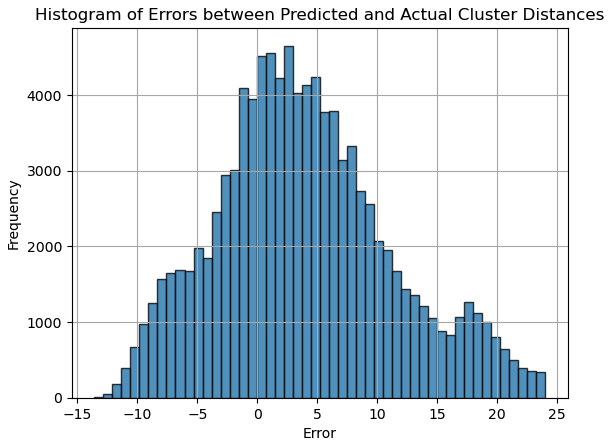
Figure 1. Histogram of Errors between Predicted and Actual Cluster Distances

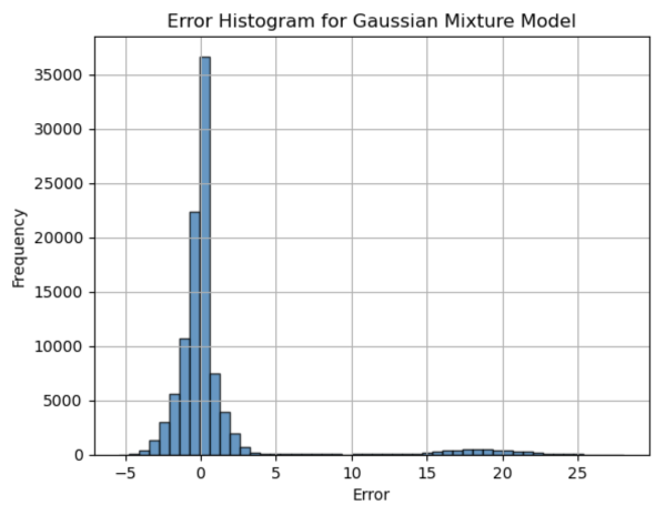
Figure 2. 1D Error Histogram for 2-cluster Gaussian Mixture Model

3.2.3. Neural Network

In the Neural Network model, we take the input data to be the histogram bin counts for each cluster [3]. The neural network is a Multi-Layer Perceptron (MLP) with input layer of 50 neurons (corresponding to 50 histogram bin counts), 3 hidden layers with 48, 100, and 100 neurons, respectively, and an output layer of 1 neuron (predicting the distance between the two cluster centers). The network is trained using the adam solver, and the loss function used is the Mean Squared Error (MSE), which measures the average of squares of the errors between the predicted and actual values.

The figure below shows the result of the Neural Network.

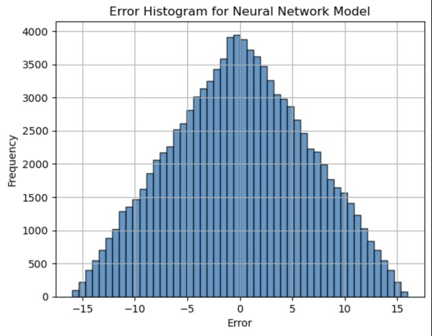
Figure 3. 1D Error Histogram for 2-cluster Neural Network

3.3. D Multiple-cluster Case

Result of different models on the 2D multiple-cluster dataset, shown by figures.

3.3.1. Center of Gravity

Describe the setup of the model in 2D case. The Center of Gravity model calculates the central point of each cluster based on the provided 2D coordinates in a text file. In this case, the “true clusters” and “found clusters” are compared to assess the model’s performance. The script processes the clusters, calculates the differences.

In the 2D multiple-cluster model, the Center of Gravity (CoG) model identifies and locate clusters by determining the local maxima within a 2D histogram. The 2D histogram’s result is generated from the provided data text file. Each cell in the histogram grind represents a bin. To determine the local maxima, we set up a hyper- parameter, which defines the neighborhood window. For a cell \( (i,j) \) with a count \( ci,j \) we can identify the local maxima if

\( {c_{i,j}} \gt {c_{i-σ,j}},…,{c_{i+σ,j}},{c_{i,j-σ}},…,{c_{i,j+σ}} \)

This can help us reduce noise by making sure that the identified cluster centers are at peaks compared to the surroundings. We processed the 2D dataset to evaluate the gap between true and predicted clusters. The overall performance of the Center of Gravity model is evaluated by comparing those differences.

3.3.2. Neural Network

Describe the setup of the model in 2D case.

In case of the 2D clusters we used a Neural Network model to predict the cluster centers that’s extracted from the 2D histogram data. And we used a Multi-Layer Perceptron (MLP) for our neural network model [4] [5].

The MLP includes the following structures; Input Layer: Flattened 64x64 grid (4096 input neurons) Hidden Layer 1: 256 neurons Hidden Layer 2: 128 neurons Hidden Layer 3: 64 neurons Output Layer: 2 neurons (predicting the x and y coordinates of the cluster center). The input of this model is the 2D histogram, and the output was the predicted coordinates and location of the cluster centers. In order to train the neural network model, we used methods such as the Adam optimizer and the Mean Squared Error (MSE) loss function. The MSE calculates the average of the squares of the errors that’s in between the predicted and true values. The overall performance of the Neural Network Model was evaluated by comparing the predicted cluster centers and the true centers.

4. Conclusion

Summarize the performances of different models (e.g. the error distribution) and discuss which is better and why. In the 1D models, the Gaussian Mixture Model per-formed the best. It had the lowest error variance and most accurate predictions, as indicated by the concentration of errors around 0 with a small group near 15 and 20. The Center of Gravity method centered around 0, but had a much larger spread of errors. This suggests that it is more susceptible to noise and less precised compared to the Gaussian Mixture Model. The Neural Network also showed a peak at 0 with a relatively symmetrical spread around it. It is less accurate than the Gaussian Mixture Model, but showed a smaller range of errors compared to the Center of Gravity Model. The Center of Gravity method can provide a reasonable cluster center prediction. It can do that by setting an appropriate, this model can identify local maxima as cluster centers effectively, it indeed is an effective method but it might be sensitive to noise and depends on the choice of. On the other hand, The Neural Network model showed an overall better performance by learning more complex spatial patterns and data from the 2D histogram data. It shows more accurate predictions of cluster centers compared to the Center of Gravity method. However, the Neural Network model requires more computational resources and more careful tuning of parameters.

5. Acknowledgement

Xiwen Gong and Zilin Zhou contributed equally to this work and should be considered co-first authors.

References

[1]. Hejazi, M. M., Golabi, F., Bahrami, M., Kahroba, H., & Hejazi, M. (2022). Fmsclusterfinder: a new tool for detection and identification of clusters of sequential motifs with varying characteristics inside genomic sequences. bioRxiv.
[2]. Feldbrugge, J., & Weygaert, R. V. D.. (2023). Cosmic web & caustic skeleton: non-linear constrained realizations 2d case studies. Journal of Cosmology and Astroparticle Physics.
[3]. Moayedi, H., Salari, M, Dehrashid, A. A. , & Le, B. N. . (2023). Groundwater quality evaluation using hybrid model of the multi-layer perceptron combined with neural-evolutionary regression techniques: case study of shiraz plain. Stochastic environmental research and risk assessment(8), 37.
[4]. Kang, H., Xu, Q., & Duofang ChenShenghan RenHui XieLin WangYuan GaoMaoguo GongXueli Chen. (2024). Assessing the performance of fully supervised and weakly supervised learning in breast cancer histopathology. Expert Systems with Application, 237(Mar. Pt.B), 121575.1-121575.13.
[5]. Wu, S., Du, Z., Zhang, F. , Zhou, Y. , & Liu, R. . (2023). Time-series forecasting of chlorophyll-a in coastal areas using lstm, gru and attention-based rnn models. Journal of Environmental Informatics.
Cite this article
Gong,X.;Zhou,Z. (2025). Cluster Finder for 1D and 2D Histogram Data. Applied and Computational Engineering,131,274-278.
Data availability
The datasets used and/or analyzed during the current study will be available from the authors upon reasonable request.
Disclaimer/Publisher's Note
The statements, opinions and data contained in all publications are solely those of the individual author(s) and contributor(s) and not of EWA Publishing and/or the editor(s). EWA Publishing and/or the editor(s) disclaim responsibility for any injury to people or property resulting from any ideas, methods, instructions or products referred to in the content.
About volume
Volume title: Proceedings of the 2nd International Conference on Machine Learning and Automation
© 2024 by the author(s). Licensee EWA Publishing, Oxford, UK. This article is an open access article distributed under the terms and
conditions of the Creative Commons Attribution (CC BY) license. Authors who
publish this series agree to the following terms:
1. Authors retain copyright and grant the series right of first publication with the work simultaneously licensed under a Creative Commons
Attribution License that allows others to share the work with an acknowledgment of the work's authorship and initial publication in this
series.
2. Authors are able to enter into separate, additional contractual arrangements for the non-exclusive distribution of the series's published
version of the work (e.g., post it to an institutional repository or publish it in a book), with an acknowledgment of its initial
publication in this series.
3. Authors are permitted and encouraged to post their work online (e.g., in institutional repositories or on their website) prior to and
during the submission process, as it can lead to productive exchanges, as well as earlier and greater citation of published work (See
Open access policy for details).