Clustering of NBA Teams Across Multiple Years

Yiming Zhong

doi:10.54254/2755-2721/2025.21716

1. Introduction

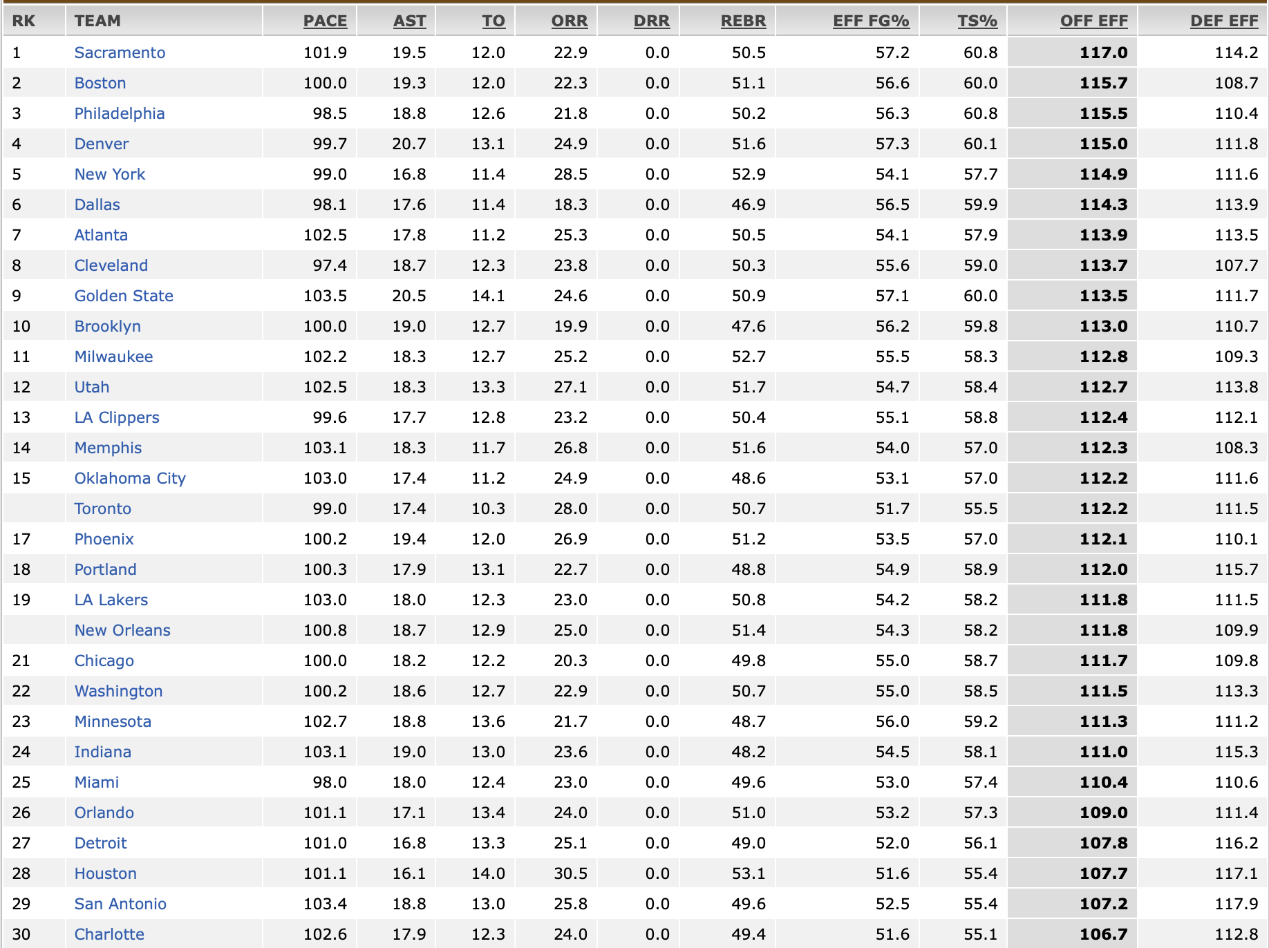
The availability of large data, improvements in computer infrastructure, and the development of machine learning have revolutionized sports analytics. Media coverage and expert studies like ESPN's have influenced sports team rankings and evaluations, such as win percentages and offensive/defensive efficiency. These rankings provide useful information, however they focus largely on win-loss records and ignore more nuanced team performance factors. Newspapers and sports media often rate teams by win % or offensive ability, but these rankings seldom account for team performance's intricacies. Figure 1 shows that current rankings, while useful, overlook important factors like the balance between offensive and defensive efficiency and the association of underlying data with sustained performance across seasons. These rankings are subjective and sometimes influenced by broad generalizations, so they don't accurately reflect a team's success across the board. Big data has given sports organizations unprecedented access to season-long insights. With advanced machine learning techniques, this data can be used to objectively evaluate teams based on win percentage, offensive efficiency, defensive efficiency, and more complex metrics like offensive-defensive strategy interaction. These data elements offer a more detailed study that goes beyond rankings and better represents a team's success. This study analyzes team performance over numerous years using machine learning methods to calculate win percentage, offensive efficiency, and defensive efficiency to address this gap. This paper focuses on:

Compare win percentages with traditional rankings to assess how well win rates align with perceived team strength.
Investigate the relationship between win percentage, offensive efficiency, and defensive efficiency, highlighting the impact of each metric on overall success.
Explore how the difference between offensive and defensive efficiencies correlates with team performance, offering a deeper understanding of the factors that drive success or failure.

To compare these characteristics to traditional rankings, we will use objective, data-driven comparisons and show the findings. The research seeks to go beyond media narratives to uncover what genuinely affects team performance.

Figure 1. 2022-2023 offense efficiency ranking

2. Data pre-analysis and methodology

2.1. Getting data

Kaggle has tons of data to train our model, providing individual stats by year and teams stats by season, including regular season and play-off conference information. ESPN, an official sports website, has annual team aggregate statistics. For this research, we utilized the ``NBA Team Stats'' data collection from Kaggle and ESPN official stats from each year. NBA has several seasons, but we will focus on the last four: 2023-2024, 2022-2023, 2021-2022, 2020-2021. We chose these 4 years since we went through covid-19, and the NBA before and after covid are really different. The NBA's status altered in 2018-2019 when Golden State Warriors lost their final. Superstars like Kevin Durant and Lebron James left. Superstar-laden teams declined as superstars left for other teams to win the crown. Before 2018-2019, a team may be ranked in the top 5 then drop to a poor team owing to superstar transfers. The player-change rate dropped after 2018-2019. This study solely considers the event following the 2018-2019 season. Additionally, we require real-world NBA franchise regular season rankings from ESPN. These data will not be used in 2.1 and 2.2. These data will be used in [???].

2.1.1. Normalization and selection of variables

Data screening and integrating data First, we must find the data type we want to use and change the numerical digits into the same range. For example, each team has a win percentage and a total free throws. We want to determine the proportion or ratio of each team's performance, rather than the overall number, as numbers are typically used to indicate individual performance rather than team performance. The NBA Team Stats dataset has a large variety of data kinds, making it difficult to assess the team's performance within a given data category. However, we may gain a perceptual intuition and compare it to other teams in the same data type by looking at the proportion. The ESPN official stats for each year have already been preprocessed, so we merely utilize their databases. Integrating NBA Team numbers and ESPN official numbers from each year provides fundamental data for research:PACE, AST, TO, ORR, DRR, REBR, EFF FG%, TS% , OFF EFF , DEF EFF, Win %, FG %, Three Point %, Free Throw %, Steals %, and Blocks %. Finally, we will receive a dataset with 30 teams and 16 variables from 2023-2024, 2022-2023, 2021-2022, and 2020-2021. Normalization After selecting data types and sets, we must preprocess our data. Since our data set has so many types and their ranges are usually varied, we need to z-score normalize it to manage the scale in each data type. Another rationale for z-score normalization. This won't be mentioned. We'll cover this in [???]. Therefore, according to z-score formula: [1]

\begin{equation} \frac{x-\mu}{\sigma} \end{equation}

where x is original value within a data type, $\mu$ is the average number within this data type, and $\sigma$ is standard deviation within this data type. By applying this formula, we will get the standardized data set.

2.2. Principal component analysis and K-means clustering [2]

2.2.1. Factors screening

Variable screening on our completed-integrating data set is required before principal component analysis (PCA). Because win %, OFF EFF, and DEF EFF determine if the team is a title contender in actual NBA games. Only the top eight teams in the East and West with the highest winning percentage will make the playoffs, and a team's regular-season winning percentage will determine its standings in either the East or West and which team it plays in the first round. OFF \& DEF EFFdetermine a team's performance. The easiest method to tell whether a team is good is by looking at their standings, or win percentage. We may next assess its OFF \& DEF EFF and other parameters. Overall, win % is the most obvious and important metric in team effectiveness. Due to their importance, these three factors will dominate PCA, obscuring other variables' occurrence. We omit those three components from PCA. Instead, we'll compare teams without those three criteria versus those with them. Our focus will be on the data set without win % vs the one with it. The data set without win %, OFF \& DEF EFF will be compared to the one with them.

2.2.2. PCA

Why using PCA? [3]
This study comprises 30 teams, each with 16 variables to define it, and each vector has 16 digits to represent its coordinate. The high-dimensional 16-variable dataset makes analysis difficult and computationally intensive. PCA reduces dimensionality by reducing variables to the primary components that capture the greatest data variation. This reduction makes the dataset manageable while keeping vital information. Many performance measures are linked in sports analytics. EFF FG % \& TR % may affect OFF EFF. Multicollinearity may distort statistical models and hide relationships. By converting correlated variables into uncorrelated principle components, PCA reduces multicollinearity and improves analysis reliability. Machine learning systems benefit from PCA data preparation. By reducing features, PCA reduces overfitting, processing, and accuracy in predictive models that predict team performance or other outcomes. Although PCA reduces variables, it keeps much of the dataset's variability. This retains critical data for analysis, preventing simplicity from losing important data insights. PCA will only be used for non-win %, OFF \& DEF EFFstatistics. The PCA is unnecessary for data that just includes win % and data that includes win %, OFF \& DEF EFF since they contain one or three tiny components.

2.2.3. K-means [4]

Why using K-means?
For projects that want to find trends in historical data without labels, K-Means is perfect. It may categorize teams by performance measures alone. Clusters help rate teams by assigning them to performance tiers. Comparing teams inside and across clusters is straightforward since they share comparable metrics. Clustering by metrics might show patterns of top-tier, mid-tier, and lower-tier teams, helping uncover what makes them successful or unsuccessful. Also, NBA statistics generally include scores, rebounds, assists, etc. By clustering teams using multidimensional metrics, K-Means makes it easier to understand which stats contribute to which rankings. K-means is a useful technique to rate teams without giving them exact standings. The team scores for each factor after PCA will be used for K-means. The key to K-means is choosing the right cluster number k. After getting the team scores for PCA, we can build a graph showing that k = 6 or 7 is appropriate for data omitting win %, offensive and defense efficiency, and win % just. We don't want k to be too little or too huge, therefore k = 6 or 7 seems reasonable. If k is too small, this classification is pointless since each group has so many teams that we can't discern any difference. If k is too high, that would be trivial and we can't have group characteristics. Choosing k = 6 or 7 makes sense. Looking at the graph, we will select k = 4 for data with just win %, OFF \& DEF EFF. We need to apply K-means for data that ``excluding win % k = 6 vs. include win % k = 4'', ``excluding win % k = 7 vs. include win % k = 4'', ``excluding win %, OFF \& DEF EFF k = 6 vs. include win %, OFF \& DEF EFF k = 4'', and ``excluding win %, OFF \& DEF EFF k = 7 vs. include win %, OFF \& DEF EFF k = 4'' for each year. After utilizing K-means, we will get each clustering result based on the dataset and k that we use.

2.3. Matching and Error Analysis

After using K-means to cluster each year, we must assess its performance. Our result alone cannot provide us the conclusion. We can't use a result as our team rating if it's not classified correctly after review. How can we define K-means' goodness? How can we define K-means to categorize teams successfully? We will use Majority Vote Error Analysis and Quantitative Error Analysis to evaluate K-means in this study. After applying K-means we will receive a dataset that includes each team and their corresponding cluster number, $$n$$ , where $n \in \mathbb{N}, n\leqslant7$ , in each dataset. We will call the K-means dataset that exclude win % $S_1^{W_k}$ and the dataset that exclude win %, OFF \& DEF EFF $S_1^{WOD_k}$ , where $k \in 6\ or\ 7$ . The data set that only include win % will be $S_2^{W}$ and the dataset that only include win %, OFF \& DEF EFF will be called $S_2^{WOD}$ .
Noted: for majority vote error analysis and quantitative error analysis, we will apply these methods for each year, which means different seasons will have different results. We will analyze different seasons separately.

2.3.1. Constructing converting functions

Considering $$S_1$$ scene:
We first construct two sets $U_6=\{A,B,C,D,E,F \}$ and $U_7=\{A,B,C,D,E,F,G \}$ .
We then construct two functions $$F^W$$ and $F^{WOD}$ :

$F^W$ : There are two mapping cases under $F^W$
2. \begin{equation} F^W: S_1^{W_6} \to U_6,\{\begin{matrix} F^W(1)=A, \textrm{if}\ n_i = 1
  F^W(2)=B, \textrm{if}\ n_i = 2
  F^W(3)=C, \textrm{if}\ n_i = 3
  F^W(4)=D, \textrm{if}\ n_i = 4
  F^W(5)=E, \textrm{if}\ n_i = 5
  F^W(6)=F, \textrm{if}\ n_i = 6
  \end{matrix}. \ \ n_i \in S_1^{W_6},\ i \in \{ 1,2,3,\dots,30\} \end{equation}
3. \begin{equation} F^W: S_1^{W_7} \to U_7,\{\begin{matrix} F^W(1)=A, \textrm{if}\ n_i = 1
  F^W(2)=B, \textrm{if}\ n_i = 2
  F^W(3)=C, \textrm{if}\ n_i = 3
  F^W(4)=D, \textrm{if}\ n_i = 4
  F^W(5)=E, \textrm{if}\ n_i = 5
  F^W(6)=F, \textrm{if}\ n_i = 6
  F^W(7)=G, \textrm{if}\ n_i = 7
  \end{matrix}. \ \ n_i \in S_1^{W_7},\ i \in \{ 1,2,3,\dots,30\} \end{equation}
$n_i$ represents the $i$ th team's corresponding cluster number.
$F^{WOD}$ : There are two mapping cases under $F^{WOD}$
2. \begin{equation} F^{WOD}: S_1^{WOD_6} \to U_6,\{\begin{matrix} F^{WOD}(1)=A, \textrm{if}\ n_i = 1
  F^{WOD}(2)=B, \textrm{if}\ n_i = 2
  F^{WOD}(3)=C, \textrm{if}\ n_i = 3
  F^{WOD}(4)=D, \textrm{if}\ n_i = 4
  F^{WOD}(5)=E, \textrm{if}\ n_i = 5
  F^{WOD}(6)=F, \textrm{if}\ n_i = 6
  \end{matrix}. \ \ n_i \in S_1^{WOD_6},\ i \in \{ 1,2,3,\dots,30\} \end{equation}
3. \begin{equation} F^{WOD}: S_1^{WOD_7} \to U_7,\{\begin{matrix} F^{WOD}(1)=A, \textrm{if}\ n_i = 1
  F^{WOD}(2)=B, \textrm{if}\ n_i = 2
  F^{WOD}(3)=C, \textrm{if}\ n_i = 3
  F^{WOD}(4)=D, \textrm{if}\ n_i = 4
  F^{WOD}(5)=E, \textrm{if}\ n_i = 5
  F^{WOD}(6)=F, \textrm{if}\ n_i = 6
  F^{WOD}(7)=G, \textrm{if}\ n_i = 7
  \end{matrix}. \ \ n_i \in S_1^{WOD_7},\ i \in \{ 1,2,3,\dots,30\} \end{equation}
$n_i$ represents the $i$ th team's corresponding cluster number.
We call each capital letters corresponding group $G_X$ , where $X \in U_6 \cup U_7$

Considering another $$S_2$$ scene: We first construct another set $L=\{a, b, c, d \}$

We then construct two functions $$f^W$$ and $f^{WOD}$ :

\begin{equation} f^W: S_2^W \to L,\{\begin{matrix} f^W(1)=a=l_1, \textrm{if}\ \mu_i = 1
f^W(2)=b=l_2, \textrm{if}\ \mu_i = 2
f^W(3)=c=l_3, \textrm{if}\ \mu_i = 3
f^W(4)=d=l_4, \textrm{if}\ \mu_i = 4
\end{matrix}. \ \mu_i \in S_2^W, i \in \{ 1,2,3,\dots,30\} \end{equation}
\begin{equation} f^{WOD}: S_2^{WOD} \to L,\{\begin{matrix} f^{WOD}(1)=a=l_1, \textrm{if}\ \mu_i = 1
f^{WOD}(2)=b=l_2, \textrm{if}\ \mu_i = 2
f^{WOD}(3)=c=l_3, \textrm{if}\ \mu_i = 3
f^{WOD}(4)=d=l_4, \textrm{if}\ \mu_i = 4
\end{matrix}. \ \mu_i \in S_2^{WOD}, i \in \{ 1,2,3,\dots,30\} \end{equation}

$\mu_i$ represents the $$i$$ th team's corresponding cluster number.
We call each lower case letters to be $l_{\mu_{i}}$ , where $l_{\mu_{i}} \in L$ .

Finally, for every $$i$$ th team under each group $$G_X$$ , we will find $$i$$ 's corresponding `` $l_{\mu_{i}}$ ''.
We let: \[G_X = \left\{ l_{\mu_{i}} \right\}\]

2.3.2. Majority voting process [5]

Define Targeting Mapping letter $$l_T$$ : For each group $$G_X$$ , we find its most frequent letter $l_{\mu_{i}}$ . We let this letter be $$l_T$$ . Noted that if there is a case that is tie, we just random choose one $l_{\mu_{i}}$ among the tie letters. We then define a function:

\begin{equation} M^V: G_X \to \{0,1 \}, M^V (G_{X_{\alpha}} )= \{\begin{matrix} 0, \textrm{if}\ l_{\mu_{i}} = l_T
1, \textrm{if}\ l_{\mu_{i}} \neq l_T \end{matrix}. \end{equation}

where $\alpha$ is the $\alpha$ th lower case letter in $$G_X$$ . After implementing this function, we basically convert each $$G_X$$ groups that contain lower case letters into $$G_X$$ groups that only contain either 0 or 1. Calculating the sum for each $$G_X$$ :

\begin{equation} Err_X = \sum_{\alpha = 1}^{| G_X|} M^V (G_{X_{\alpha}}) \end{equation}

Finally, we calculate the percent error:

\begin{equation} Perc^{M} = \frac{\sum_{X}^{}Err_X}{N} \cdot 100% \end{equation}

where $$N = 30$$ in this case.

2.3.3. Quantitative error process

The quantitative error process involves a more detailed numerical approach to evaluating cluster quality. Instead of relying solely on the frequency of subcategories like majority voting process,this method leverages numerical rankings and distance-based evaluations to offer a nuanced understanding of classification performance. In this section we need to use the regular season team standing dataset as we mentioned in 2.1. Define Mapping axis:
For the teams that have the same $l_{\mu_{i}}$ , we find its corresponding team's position $$r_i$$ in corresponding regular season standing dataset. We said this set for the teams that have the same $l_{\mu_{i}}$ to be $T_{l_{\mu_{i}}}$ ,

\begin{equation} Avg T_{l_{\mu_{i}}}= (\sum_{\beta=1}^{|T_l |} r_{i_{\beta}}) \cdot \frac{1}{|T_l |} \end{equation}

where $\beta$ means the $\beta$ th element in $T_{l_{\mu_{i}}}$ . We will get an average standing for each $l_{\mu_{i}}$

$(\textrm{i.e.\ each ``a, b, c, d''})$ . Then we sort them from the smallest to the largest. We assign each lower case letter a number 1, 2, 3, 4 from the lowest to the largest. (i.e. if $AvgT_a \lt AvgT_b \lt AvgT_c \lt AvgT_d$ , then $a \to 1, b \to 2, c \to 3, d \to 4$ )
Define ``distance'': For each $$G_X$$ , we calculate the distance for all four possible mappings of lower case letters for every $l_{\mu_{i}}$ in $$G_X$$ . For each mapping $l_m \in \{a, b, c, d \}$ :

\begin{equation} D_{G_{X},l_{\mu_{i}}} = \sum (x_{\mu{i}}-x_{l_{m}})^2 \end{equation}

where $x_{\mu{i}}$ means the corresponding sorting number on mapping axis. $x_{l_{m}}$ means the corresponding sorting number on mapping axis. For each $$G_X$$ , we can compare the distances based on different mapping $$l_m$$ :

\begin{equation} D_{X_{min}} = Min(D_{G_{X},l_{\mu_{i}}}) \end{equation}

After this process, we will get different distances between $$S_1$$ and $$S_2$$ for each $$G_X$$ . Finally, we can calculate the total distance and percent error:

\begin{equation} D_{total} = \sum D_{X_{min}} \end{equation}

\begin{equation} Perc^{Q}= \frac{D_{total}}{N} \cdot 100% \end{equation}

3. Results and visualizations

3.1. PCA and visualizations of clusters

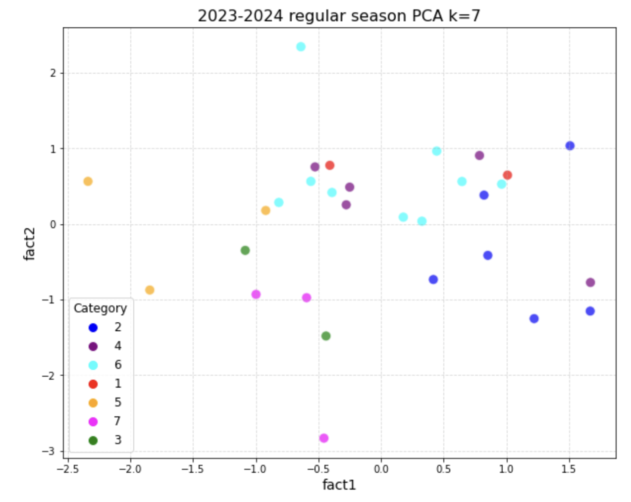
We won't include four years' visualization since each year will have two cases: exclude win % solely and exclude win %, OFF \& DEF EFF. We will have k=6 and k=7 examples for these two scenarios. Putting all the visualization graphs here will take up a lot of material. Thus, in 3.1, we will show using the 2023-2024 regular season and results.

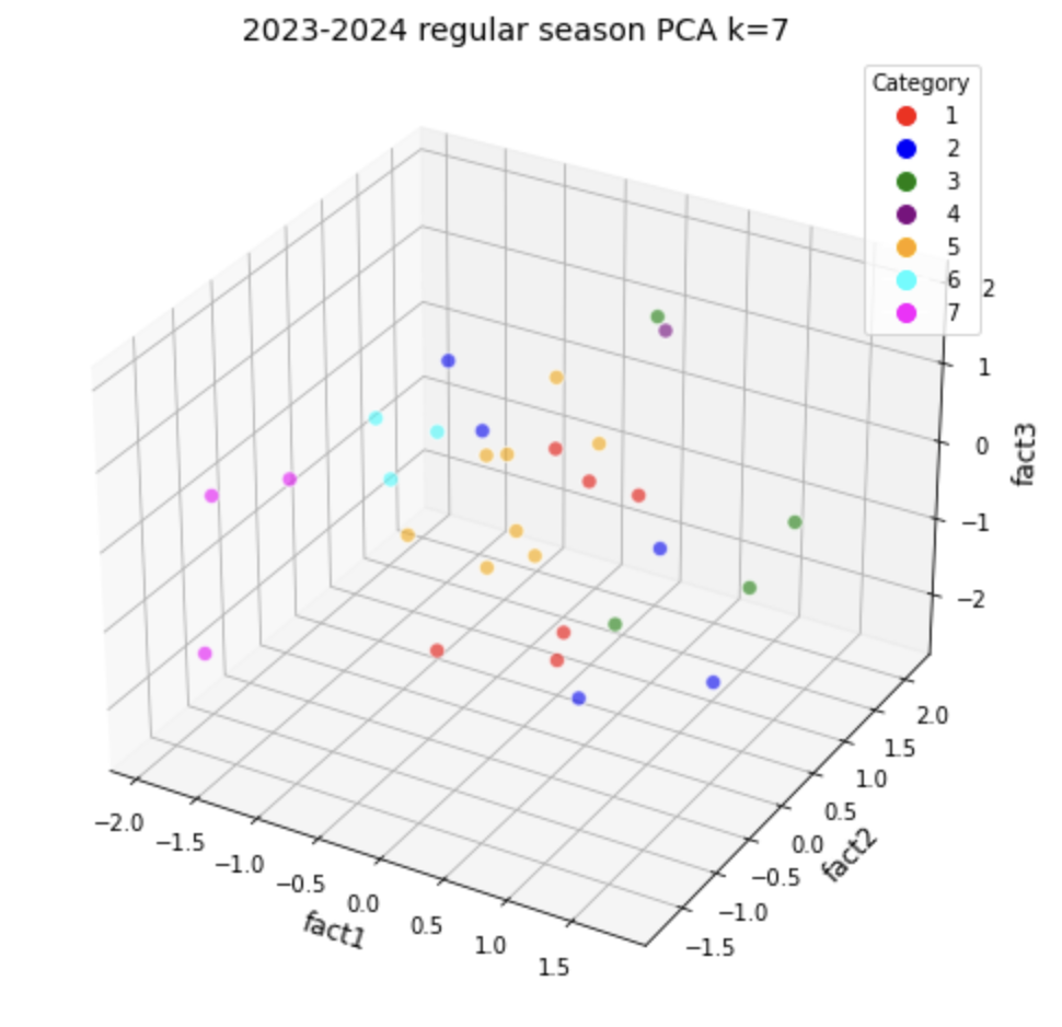
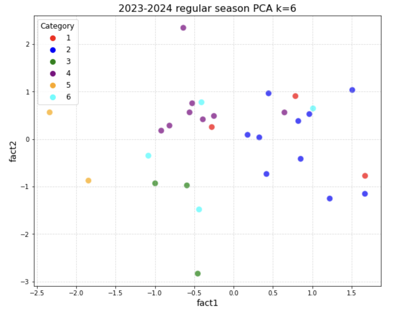
3.1.1. Visualization of $S_1^{W_k}$ with its PCA data

After we implemented PCA method, we would reduce the total factors from 16 to 5 factors in this case. However, we can't draw a graph that contains 5 coordinates in graph, so we split those 5 factors into 3 factors a graph and 2 factors a graph.
When cluster k = 6:

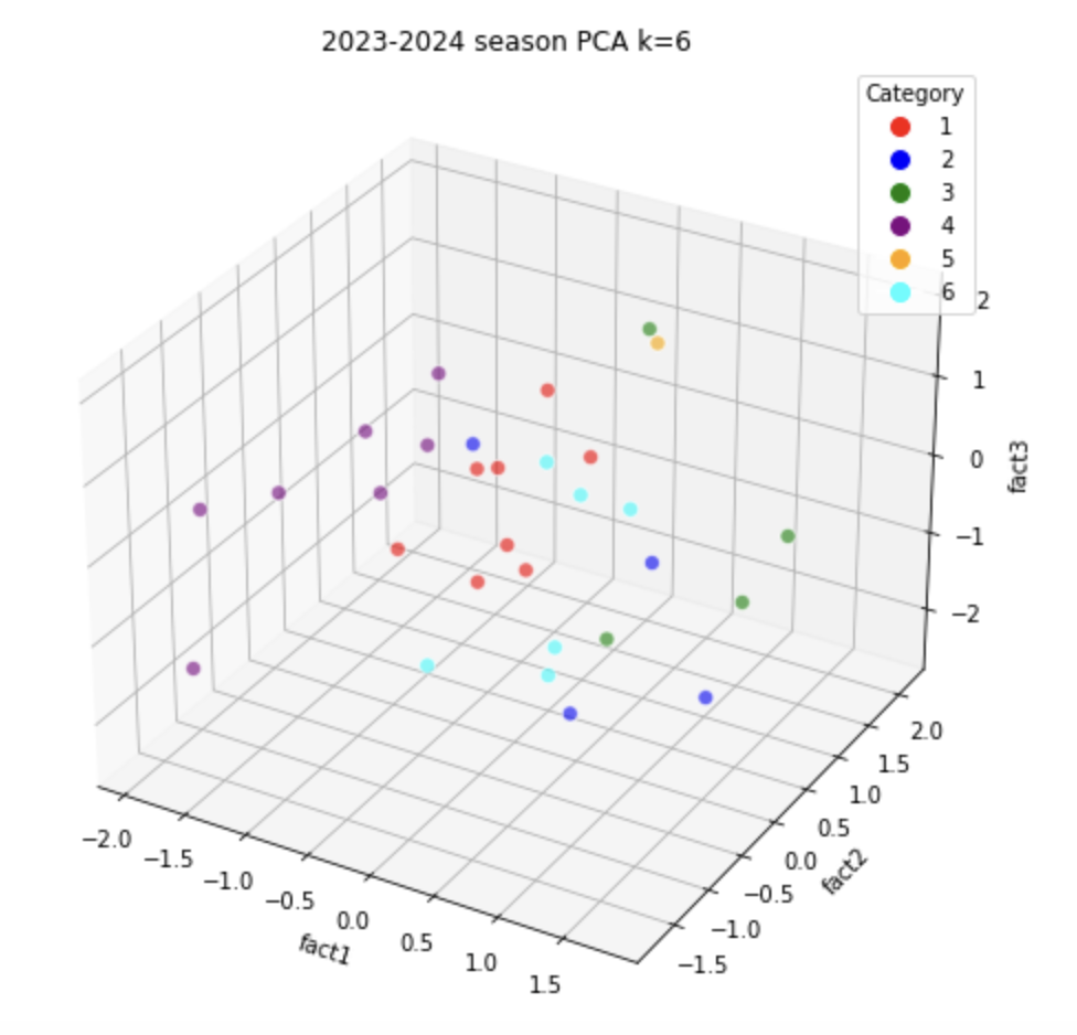
Figure 2. Visualization of $S_1^{W_6}$ with its PCA data when k = 6

When cluster k = 7:

Figure 3. Visualization of $S_1^{W_6}$ with its PCA data when k = 7

3.1.2. Visualization of $S_1^{WOD_k}$ with its PCA data

In $S_1^{WOD_k}$ , after we implemented PCA, we will reduce the total factors from 16 to 4. Therefore, we will split these 4 factors into 2 factors a graph separately. When cluster k = 6:

Figure 4. Visualization of $S_1^{WOD_6}$ with its PCA data when k = 6

When cluster k = 7:

Figure 5. Visualization of $S_1^{WOD_7}$ with its PCA data when k = 7

3.2. Matching and values of error

Same as 3.1, in this section we will only show one year's matching result and its corresponding values of error. In this section we will choose 2021-2022 regular season to show some of the results and its values of error.

3.2.1. Majority voting error analysis

Results of $S_1^{W}$ vs. $$S_2^W$$

When cluster k = 7:

Table 2. Results of K-means when k = 7 for $$S^W$$

Team	Cluster number in $$S_1^W$$	Cluster number in $$S_2^W$$
Atlanta	1	2
Utah	5	2
Phoenix	7	3
Milwaukee	7	2
Boston	5	2
Denver	5	2
Charlotte	7	2
Memphis	3	3
Minnesota	7	2
Miami	5	2
Philadelphia	1	2
Chicago	1	2
Brooklyn	7	2
Dallas	5	2
Golden State	5	2
Toronto	2	2
San Antonio	7	1
Cleveland	5	1
Indiana	7	2
New Orleans	5	4
Washington	2	1
New York	1	1
LA Lakers	2	1
LA Clippers	7	2
Sacramento	1	2
Portland	7	1
Houston	4	4
Detroit	6	4
Oklahoma City	4	4
Orlando	4	4

Implementing function

\(F^W\)

and

\(f^W\)

:
Group A (A): Atlanta: b, Boston: b, Denver: a, Miami: b
Do the same way for Group B C D E F G. We will get

\(l_T\)

for each group:

\(G_A\)

: b \

\(G_B\)

: a \

\(G_C\)

: c \

\(G_D\)

: d \

\(G_E\)

: b \

\(G_F\)

: d \

\(G_G\)

: b Implementing functions

\(M^V\)

\(Err_X\)

, and

\(Perc^M\)

\frac{1+1+0+0+0+0+5}{30} \cdot 100% = 23.3%

When k = 6, $$Perc^M$$ = $\frac{1+1+5+0+2+0}{30} \cdot 100% = 30%$

Results of $S_1^{WOD}$ vs. $S_2^{WOD}$

When cluster k = 6:
$$l_T$$ for each group: $$G_A$$ : a \ $$G_B$$ : d \ $$G_C$$ : d \ $$G_D$$ : c \ $$G_E$$ : b \ $$G_F$$ : a $$Perc^M$$ = $\frac{6+0+1+0+0+4}{30} \cdot 100% = 36.67%$
When cluster k = 7 $$l_T$$ for each group: $$G_A$$ : a \ $$G_B$$ : d \ $$G_C$$ : a \ $$G_D$$ : c \ $$G_E$$ : b \ $$G_F$$ : a \ $$G_G$$ : d $$Perc^M$$ = $\frac{4+1+3+0+0+3+0}{30} \cdot 100% = 36.67%$

3.2.2. Quantitative error analysis

In this section, we will not show the converting results since we have already showed in [???] and [???]. We will only show the the process and results in quantitative error analysis. We need to use 2021-2022 regular season standings data in this part. Since we need to use this dataset all the time, we just show this data in the front:

Table 1: 2021-2022 regular season standings

Team name	Standing
Phoenix Suns	1
Memphis Grizzlies	2
Miami Heat	3
Golden State Warriors	4
Dallas Mavericks	5
Boston Celtics	6
Milwaukee Bucks	7
Philadelphia 76ers	8
Utah Jazz	9
Toronto Raptors	10
Denver Nuggets	11
Minnesota Timberwolves	12
Chicago Bulls	13
Brooklyn Nets	14
Cleveland Cavaliers	15
Atlanta Hawks	16
Charlotte Hornets	17
LA Clippers	18
New York Knicks	19
New Orleans Pelicans	20
Washington Wizards	21
San Antonio Spurs	22
Los Angeles Lakers	23
Sacramento Kings	24
Portland Trail Blazers	25
Indiana Pacers	26
Oklahoma City Thunder	27
Detroit Pistons	28
Orlando Magic	29
Houston Rockets	30

Results of $S_1^{W}$ vs. $$S_2^W$$ Since mapping axis only has difference between different $$S_2$$ (i.e. $$S_2^W$$ and $S_2^{WOD}$ ), within the same $$S_2$$ , we can calculate the mapping axis first. Finding Mapping axis:
{Lowercase Letter ``a'':}

$Avg T_{a}$ = Washington Wizards (21) + Sacramento Kings (24) + San Antonio Spurs (22) + LA Lakers (23) + New Orleans Pelicans (20) + New York Knicks (19) $$/ 6 = 21.5$$

Same way as ``b'': 10.5, ``c'': 1.5, ``d'': 27.5.
Axis: 1 $\to$ c, 2 $\to$ b, 3 $\to$ a, 4 $\to$ d

When cluster k = 6:
Implementing functions $D_{G_{X},l_{\mu_{i}}}$ , $D_{X_{min}}$ , and $D_{total}$ :
{Group A (A):} Lowercase Letters: b, b, b, b, b, b, b, a, b
Mapping A to c (1):
2. Distances:
3. b: $$ (2 - 1)^2 = 1 $$ (for 8 teams)
4. a: $$ (3 - 1)^2 = 4 $$ (for 1 team)
Total Distance: $(1 \times 8) + (4 \times 1) = 12$ Do the same way for mapping A to b, c, d, then we get: 1, 8, 33. So the minimum distance for A is 1 (mapping to b).
We then do the rest of the group B, C, D, E, F and we get the minimum distances are 1, 7, 0, 2, 0. So $$Perc^Q$$ = $\frac{1+1+7+0+2+0}{30} \cdot 100% = 36.67 %$
When cluster k = 7:
$$Perc^Q$$ = $\frac{10}{30} \cdot 100% = 33.3%$

Results of $S_1^{WOD}$ vs. $S_2^{WOD}$ Axis: c → 1, a → 2, d → 3, b → 4

When cluster k = 6:
$$Perc^Q$$ : $\frac{ 6 + 0 + 1 + 0 + 0 + 7}{30} \cdot 100% \approx 46.67%$
When cluster k = 7:
$$Perc^Q$$ : $\frac{4 + 1 + 6 + 0 + 0 + 3 + 0}{30} \cdot 100% \approx 46.67%$

4. Conclusion

This data-driven study used Principal Component Analysis (PCA) and K-Means clustering to evaluate NBA team rankings objectively. The research used previous NBA seasons to emphasize win percentage, offensive efficiency, and defensive efficiency, as well as multidimensional performance measurements. The results show that grouping NBA teams by PCA-reduced variables showed performance tiers that standard ranking algorithms miss. Teams with good OFF \& DEF stats concentrated in top-performing groupings, matching their high win percentages. PCA simplifies understanding and preserves variance by reducing dimensionality of complicated datasets. K-Means clustering effectively distinguishes team levels with k-values of 6 or 7. Quantitative and majority voting error analysis confirmed clustering results. In various setups, majority voting error rates varied from 23.3% to 36.67%, whereas quantitative mistakes indicated clustering accuracy from 33.3% to 46.67%. These findings showed team classification's balance between simplicity and accuracy. This study goes beyond win-loss statistics to assess NBA team performance with a sophisticated analytical methodology. The findings improve sports analytics by helping assess teams and make strategic decisions. For larger applications, future study might incorporate player-specific metrics or apply similar methods to other sports leagues.

5. Pros and cons

Pros:

Objectivity: This method minimized biases inherent in traditional rankings by relying on data-driven analysis.
Multidimensionality: Incorporating diverse metrics provided a comprehensive understanding of team performance.
Scalability: The approach can be applied across multiple seasons or extended to other sports leagues.

Cons:

Simplification of metrics: The exclusion of key metrics like win percentage during PCA analysis, while necessary for reducing redundancy, may overlook some intuitive aspects of team rankings.
Cluster rigidity: The K-Means clustering method assumes predefined cluster numbers (k), which may not always align perfectly with real-world team dynamics.
Error sensitivity: Results depend on the quality of the dataset and preprocessing steps like normalization, making the method sensitive to data imperfections.

6. Future directions

Hierarchical Clustering: Future work could explore hierarchical clustering [6] to identify nested group structures, offering insights into relationships between team tiers.
Incorporating Temporal Analysis: A time-series approach could be employed to track team performance trends over several seasons.
Integration of Player-Level Data: Adding individual player metrics, such as player efficiency ratings and injury history, could enhance the analysis of team dynamics.
Enhanced Validation Techniques: Cross-validation methods or comparison with alternative clustering algorithms (e.g., DBSCAN [7] or Gaussian Mixture Models [8]) could strengthen the robustness of findings.

References

[1]. Michal S Gal and Daniel L Rubinfeld. Data standardization. NYUL Rev., 94:737, 2019.

[2]. Marija Norusis. SPSS 15.0 guide to data analysis. Prentice Hall Press, 2007.

[3]. Andrzej Mac ́kiewicz and Waldemar Ratajczak. Principal components analysis (pca). Computers & Geosciences, 19(3):303–342, 1993.

[4]. Tapas Kanungo, David M Mount, Nathan S Netanyahu, Christine D Piatko, Ruth Silverman, and Angela Y Wu. An efficient k-means clustering algorithm: Analysis and implementation. IEEE transactions on pattern analysis and machine intelligence, 24(7):881–892, 2002.

[5]. Robert S Boyer and J Strother Moore. Mjrty—a fast majority vote algorithm. In Automated reasoning: essays in honor of Woody Bledsoe, pages 105–117. Springer, 1991.

[6]. Fionn Murtagh and Pedro Contreras. Algorithms for hierarchical clustering: an overview. Wiley Interdisciplinary Reviews: Data Mining and Knowledge Discovery, 2(1):86–97, 2012.

[7]. ErichSchubert,Jo ̈rgSander,MartinEster,HansPeterKriegel,andXiaoweiXu.Dbscanrevisited, revisited: why and how you should (still) use dbscan. ACM Transactions on Database Systems (TODS), 42(3):1–21, 2017.

[8]. Douglas A Reynolds et al. Gaussian mixture models. Encyclopedia of biometrics, 741(659-663), 2009.

Cite this article

Zhong,Y. (2025). Clustering of NBA Teams Across Multiple Years. Applied and Computational Engineering,119,122-134.

Data availability

The datasets used and/or analyzed during the current study will be available from the authors upon reasonable request.

Disclaimer/Publisher's Note

The statements, opinions and data contained in all publications are solely those of the individual author(s) and contributor(s) and not of EWA Publishing and/or the editor(s). EWA Publishing and/or the editor(s) disclaim responsibility for any injury to people or property resulting from any ideas, methods, instructions or products referred to in the content.

About volume

Volume title: Proceedings of the 3rd International Conference on Software Engineering and Machine Learning

ISBN：978-1-83558-805-5(Print) / 978-1-83558-806-2(Online)

Editor：Marwan Omar, Hui-Rang Hou

Conference website: https://2025.confseml.org/

Conference date: 2 July 2025

Series: Applied and Computational Engineering

Volume number: Vol.119

ISSN：2755-2721(Print) / 2755-273X(Online)

© 2024 by the author(s). Licensee EWA Publishing, Oxford, UK. This article is an open access article distributed under the terms and conditions of the Creative Commons Attribution (CC BY) license. Authors who publish this series agree to the following terms:
1. Authors retain copyright and grant the series right of first publication with the work simultaneously licensed under a Creative Commons Attribution License that allows others to share the work with an acknowledgment of the work's authorship and initial publication in this series.
2. Authors are able to enter into separate, additional contractual arrangements for the non-exclusive distribution of the series's published version of the work (e.g., post it to an institutional repository or publish it in a book), with an acknowledgment of its initial publication in this series.
3. Authors are permitted and encouraged to post their work online (e.g., in institutional repositories or on their website) prior to and during the submission process, as it can lead to productive exchanges, as well as earlier and greater citation of published work (See Open access policy for details).

References

[1]. Michal S Gal and Daniel L Rubinfeld. Data standardization. NYUL Rev., 94:737, 2019.

[2]. Marija Norusis. SPSS 15.0 guide to data analysis. Prentice Hall Press, 2007.

[3]. Andrzej Mac ́kiewicz and Waldemar Ratajczak. Principal components analysis (pca). Computers & Geosciences, 19(3):303–342, 1993.

[5]. Robert S Boyer and J Strother Moore. Mjrty—a fast majority vote algorithm. In Automated reasoning: essays in honor of Woody Bledsoe, pages 105–117. Springer, 1991.

[6]. Fionn Murtagh and Pedro Contreras. Algorithms for hierarchical clustering: an overview. Wiley Interdisciplinary Reviews: Data Mining and Knowledge Discovery, 2(1):86–97, 2012.

[8]. Douglas A Reynolds et al. Gaussian mixture models. Encyclopedia of biometrics, 741(659-663), 2009.