1. Introduction

1.1. Reinforcement Learning

Reinforcement learning (RL) is a branch of machine learning where the core idea is that an agent (AI) learns by interacting with an environment through trial and error, receiving rewards (positive or negative) as feedback for its actions. The agent aims to maximize the reward by taking the correct actions and thus finding the optimal decision-making strategy.

During the execution of reinforcement learning, the agent interacts with the environment by receiving the current state \( {s_{t}} \) , performing an action \( {a_{t}} \) based on this state, and then receiving a reward \( {r_{t}} \) and a new state \( {s_{t+1}} \) from the environment in response to the action.

Compared to other machine learning methods, supervised learning uses labeled data for learning, unsupervised learning discovers patterns and inherent structures in unlabeled data, while reinforcement learning uses unlabeled data, but the agent can determine if it is closer or farther from the goal based on reward feedback, learning from a series of reinforcement—rewards or punishments [1].

1.2. Autonomous Driving

Autonomous driving is the ability of a vehicle to sense its environment, plan its path, and drive safely and autonomously without human intervention using artificial intelligence, sensors, computer vision, and control systems. Its core objectives are to enhance traffic efficiency, reduce accidents, and free up human driving time [2].

Autonomous driving relies on the integration of multiple technologies, such as environmental perception through multi-sensor fusion, including LiDAR, cameras, and millimeter-wave radar, to achieve 360° coverage with no blind spots [3]; path planning and decision-making using a hybrid architecture of deep learning and rule-based engines [4]; and precise control of steering, throttle, and braking using Model Predictive Control (MPC) and steer-by-wire technologies [5]. Compared to human driving, autonomous driving has many advantages, such as faster response times in milliseconds, the ability to stay focused without fatigue or emotional interference, making it suitable for long-distance driving tasks [6]; and while humans may have visual blind spots, autonomous driving can achieve 360° coverage using multi-sensor fusion [3].

1.3. Current Progress in Reinforcement Learning and Autonomous Driving

In recent years, reinforcement learning has been significantly integrated into autonomous driving, such as through Q-Learning, DQN, and PPO, using high-precision maps and real-time perception data for decision-making and path planning in scenarios like lane changes, overtaking, and intersections [7]. Multi-agent reinforcement learning (MARL) methods, like MADDPG, simulate complex traffic flows to predict pedestrian and vehicle intentions and optimize interaction strategies [8]. By combining Model Predictive Control (MPC) with reinforcement learning algorithms like SAC, these systems balance comfort and energy consumption, enabling smooth control of throttle, brakes, and steering.

However, current research primarily focuses on single-objective optimization, such as maximizing either driving efficiency or safety. There is relatively little research on multi-objective optimization (MOO), which is essential as real-world driving tasks typically require the optimization of multiple conflicting objectives, such as safety, efficiency, comfort, and energy consumption.

1.4. Our Work

This paper proposes a reward function design method aimed at balancing safety and efficiency. We use reinforcement learning (PPO algorithm) to train seven autonomous driving models in the MetaDrive simulation environment to complete driving tasks safely and efficiently. After training, the models are evaluated, including automatic generation of JSON-format test reports and saving driving process animations categorized by turning type. Based on the generated test reports, we calculate the success rates and average frame counts required for each model in various turning scenarios, thus analyzing the results.

2. Related work

2.1. Challenges in Designing Reward Functions for Reinforcement Learning

In reinforcement learning, the design of the reward function directly determines the agent's learning objectives and behavioral strategies. However, in complex scenarios such as autonomous driving, significant challenges arise, particularly in balancing safety and efficiency.

2.1.1. Challenges in Reward Function Design

In autonomous driving, the reward function depends not only on the current state and action but also on time, driving scenarios, traffic conditions, and other complex factors. Moreover, autonomous driving tasks often require reward functions that balance multiple objectives, which are often conflicting. For example, cautious driving reduces risk but increases travel time, while high-speed driving reduces travel time but increases risk. The linear weighting in reward functions is limited because static weights cannot adapt to dynamic scenarios, and fixed weights can lead to suboptimal strategies [9]. Sparse rewards are a common problem in the reinforcement learning training process, where the agent may receive insufficient feedback over long periods, causing instability in the learning process. In autonomous driving, key events like reaching the destination or crashing rarely occur in the early stages of training, resulting in slow learning [10]. Moreover, the manual design of reward functions is subjective, which can lead to reward shaping biases. For example, if we reward a specific behavior too much, the agent may focus excessively on that behavior, leading to overfitting to certain scenarios and ultimately suboptimal strategies [11].

2.1.2. Challenges in Balancing Safety and Efficiency

There is little research that designs reward functions specifically to balance safety and efficiency, as these two goals often conflict in real-world driving scenarios. First, safety is very difficult to quantify. The risk of a crash is non-linearly related to factors such as vehicle speed and distance, making it difficult to model using simple reward terms [12]. Additionally, efficiency metrics present a short-term vs. long-term conflict. Greedy optimizations for immediate efficiency (e.g., frequent lane changes) may accumulate long-term risks, with short-term efficiency improvements coming at the cost of long-term safety [13].

2.2. Importance of Multi-Objective Optimization in Autonomous Driving

Multi-objective optimization in autonomous driving refers to the simultaneous consideration and optimization of multiple conflicting objectives in the design of autonomous driving systems.

2.2.1. Importance of Multi-Objective Optimization

In real-world environments, these objectives often conflict with each other. Therefore, multi-objective optimization is crucial for improving the performance of autonomous driving systems and is necessary for the practical deployment of autonomous driving technology. Multi-objective optimization enables the system to make more comprehensive and accurate decisions, improving overall performance and user experience. In complex traffic environments, it helps the autonomous system handle dynamic changes more effectively, ensuring the system can adapt to a wide range of traffic scenarios. Through multi-objective optimization, the system can maintain stable performance under different conditions, reducing the limitations of single-objective optimization and improving reliability and stability. If multi-objective optimization is neglected, strategies may overfit to a single goal and fail in complex scenarios, thus failing to meet users' needs for comprehensive driving experiences.

2.2.2. Limitations of Past Single-Objective Optimization Research

Ziegler et al. focused on optimizing efficiency by minimizing travel time. However, by prioritizing speed and aggressive path planning, their approach sometimes led to safety risks in complex traffic scenarios. The lack of safety awareness in single-objective optimization makes it unsuitable for real-world deployment [14]. Bojarski et al. developed an end-to-end deep learning model that prioritizes lane-keeping safety but does not optimize passenger comfort or traffic efficiency. Although the system performs well in structured environments, it struggles in dynamic interactions like merging and overtaking, highlighting the need to balance safety and confidence [15]. Ohn-Bar et al. focused on minimizing acceleration and jerk to optimize ride comfort, but this led to overly cautious driving behavior and poor navigation efficiency in urban environments. This indicates the need for multi-objective optimization to consider both comfort and travel time efficiency [16].

3. Our method

3.1. Components of the Reward Function

This paper designs a reward function aimed at balancing safety and efficiency. Here, we provide a detailed explanation of the components of the reward function.

3.1.1. Penalty for Wrong-Way Driving

\( reward -= self.config.get("wrong\_way\_penalty", 50.0) \) (1)

First, we check if the vehicle is driving on the wrong-way lane. If the vehicle is moving in the wrong direction on a one-way lane, a fixed penalty is applied (default value: 50). The wrong-way driving penalty forces the vehicle to follow traffic rules, optimizing safety.

3.1.2. Reward for Forward Distance

\( reward+=self.config.get("driving\_reward",1.0)*(long\_now-long\_last)*positive\_road \) (2)

Firstly, obtain the front and rear positions ( \( long\_last \) and \( long\_now \) ) of the vehicle in the lane coordinate system to calculate the position change of the vehicle in the lane: \( long\_now - long\_last \) , multiply by the positive coefficient ( \( positive\_road \) ) again to prevent obtaining positive rewards when driving in the opposite direction, with a weighted coefficient ( \( driving\_reward \) ) value of 1.0. The forward distance reward is used to encourage vehicles to continue moving along the lane direction, optimizing efficiency.

3.1.3. Speed Reward

\( reward += self.config.get("speed\_reward", 0.1) * speed\_factor * positive\_road \) (3)

Firstly, calculate the speed factor: \( speed\_factor = vehicle.speed\_km\_h / vehicle.max\_speed\_km\_h \) , multiplying by the positive coefficient ( \( positive\_road \) ), the weighted coefficient ( \( speed\_reward \) ) value is 0.1. Speed reward is used to encourage vehicles to maintain a reasonable speed (close to the speed limit), but not excessively pursue high speeds, optimizing efficiency.

3.1.4. Termination Condition Handling

3.1.4.1. Success Reward

\( reward += 40 \) (4)

If the vehicle successfully reaches the destination, a fixed reward of 40 is applied. This success reward encourages the vehicle to complete the driving task safely, optimizing safety.

3.1.4.2. Collision Penalty

Table 1: Collision Penalty Reward Functions for Models 1~7.

If the vehicle crashes, as shown in Table 1, fixed penalties (20, 10, 30 respectively) will be applied to Model 2, Model 3, and Model 4; The penalty values of Model 1, Model 5, Model 6, and Model 7 are directly proportional to the vehicle speed at the time of collision (0.2 * speed, 0.1 * speed, 0.3 * speed, 10+0.1 * speed, respectively). High-speed crashes incur higher penalties, which better reflect actual risks. Collision penalty is used to prevent crashes and optimize both safety and efficiency.

3.1.4.3. Other Termination Penalty

\( reward -= 20 * 1.2 \) (5)

If the vehicle terminates due to non-successful or crash-related outcomes, such as going off-road, a fixed penalty (default 20 * 1.2=24) is applied. This penalty prevents the vehicle from going out of bounds, optimizing safety.

3.2. Training Method (PPO)

3.2.1. Core Principle of PPO

Proximal Policy Optimization (PPO) is an on-policy reinforcement learning algorithm based on policy gradients. Its core idea is to limit the magnitude of policy updates to avoid overly deviating from the current policy, thus ensuring training stability. PPO defines a clipping objective to restrict the ratio of policy updates within a trust region ( \( [1-ϵ, 1+ϵ] \) ) to avoid excessive changes.

3.2.2. PPO Objective Function

The objective of PPO is to maximize the expected return of a policy. PPO uses the following objective function to ensure stable updates:

\( {L^{CLIP}}(θ)={\hat{E}_{t}}[min({r_{t}}(θ){\hat{A}_{t}},clip⁡({r_{t}}(θ),1-ϵ,1+ϵ){\hat{A}_{t}})] \) (6)

\( {r_{t}}(θ)=\frac{{π_{θ}}({a_{t}}|{s_{t}})}{{π_{{θ_{old}}}}({a_{t}}|{s_{t}})} \) is the policy ratio, representing the ratio between the current policy and the old policy. \( {\hat{A}_{t}} \) is the advantage function of time step \( t \) , which measures the quality of the current action relative to the average action. \( ϵ \) is a hyperparameter used to control the clipping range.

The key to this objective function is to limit the magnitude of policy updates through clipping operations. When the ratio \( {r_{t}}(θ) \) falls within the range of \( [1-ϵ, 1+ϵ] \) , the objective function will revert to the conventional policy gradient form, maximizing the advantage function; When the ratio exceeds this range, the objective function will be clipped to avoid excessive policy updates.

3.2.3. Advantage Function Calculation

The PPO algorithm uses the advantage function to estimate the relative value of a certain action, which then guides the optimization of the strategy. The advantage function typically uses Generalized Advantage Estimation (GAE) to reduce variance and improve estimation accuracy. The GAE formula is:

\( {\hat{A}_{t}}={δ_{t}}+(γλ){δ_{t+1}}+(γλ{)^{2}}{δ_{t+2}}+… \) (7)

\( {δ_{t}}={r_{t}}+γV({s_{t+1}})-V({s_{t}}) \) is the time difference error (TD error) of time step \( t \) , \( γ \) is the discount factor, and \( λ \) is the hyperparameter of GAE.

3.2.4. PPO Training Process

3.2.4.1. Sampling Data

The agent interacts with the environment and collects trajectory data over time (states, actions, rewards, etc.).

3.2.4.2. Calculating Advantage Function

Use methods like GAE to compute the advantage function \( {\hat{A}_{t}} \) ​ for each time step.

3.2.4.3. Updating the Policy

Use PPO's objective function (clipped strategy) to update the policy parameters. Each update involves multiple small steps of gradient ascent to optimize the objective function.

3.2.4.4. Updating the Value Function

Optimize the state value function by minimizing the mean squared error (MSE) of the value function, typically using the objective function \( {L^{VF}}(θ)={E_{t}}[({V_{θ}}({s_{t}})-{\hat{V}_{t}}{)^{2}}] \) to train the value function.

4. Experiment Result

4.1. Hyperparameter Settings

4.1.1. Environment Configuration Hyperparameters

Table 2: Environment Configuration Hyperparameters.

4.1.2. PPO Algorithm Hyperparameters

Table 3: PPO Algorithm Hyperparameters.

4.2. Results Analysis

In the case of a collision, Models 2, 3, and 4 apply fixed penalties (20, 10, and 30, respectively), which are fixed penalty models. Models 1, 5, 6, and 7 have penalties that are proportional to the vehicle's speed in the event of a collision (0.2 * speed, 0.1 * speed, 0.3 * speed, and 10 + 0.1 * speed, respectively), which are dynamic penalty models. The results of Models 1~7 are analyzed in terms of safety (success rate) and efficiency (average number of frames required to complete the task).

Figure 1 shows the training results for the models with different reward functions. Specifically, it illustrates how the average reward of each model changes with the training steps/episodes. The x-axis represents the training steps (or episodes), and the y-axis shows the average reward per training episode.

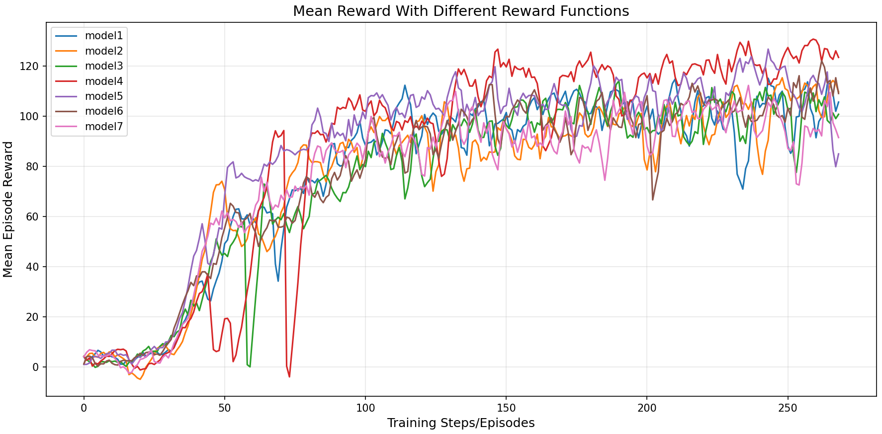
Figure 1: Mean Reward with Different Reward Functions.

From Figure 1, it can be seen that as training progresses, the average reward for each model gradually increases. This indicates that as the models interact with the environment, they learn more effective strategies, leading to higher rewards.

The success rate for each model in various turning scenarios is shown in Table 4.

Table 4: Success Rate.

The average number of frames required to complete the task for each model in different turning scenarios is shown in Table 5.

Table 5: Average Number of Frames to Complete the Task.

Figures 2, 3, and 4 show the relationship between success rate and average frames required to complete the task for different models in various turning scenarios. In these figures, the left y-axis represents the success rate, and the right y-axis represents the average number of frames to complete the task. The x-axis represents different models (Models 1 to 7). By comparing the performance of the different models in these two metrics, we can analyze their safety and efficiency in different turning types.

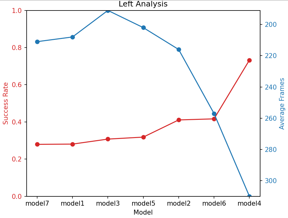
Figure 2: Left Analysis.

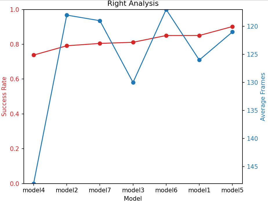
Figure 3: Right Analysis.

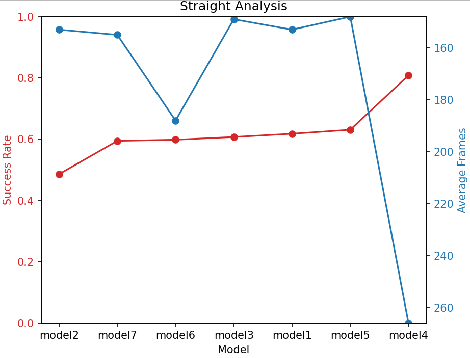
Figure 4: Straight Analysis.

Model 1 performs well in terms of safety and efficiency during right turns but performs poorly in terms of safety during left turns. Model 2 shows good efficiency but poor safety due to insufficient penalty, leading to frequent risky lane changes. Model 3 shows high efficiency during left turns but poor safety, resulting in high risk and low returns. Model 4 has the best safety in both left and straight turns, though its safety during right turns is relatively poor. However, it is the least efficient across all turning types, as high fixed penalties promote conservative driving, significantly reducing collisions but sacrificing efficiency. Model 5 strikes a good balance between safety and efficiency during right turns and straight driving, as the penalties dynamically adjust based on the vehicle’s speed. This model helps avoid high-speed collisions and prevents overly cautious driving. However, its safety during left turns is lower. Model 6 performs well in terms of both safety and efficiency during right turns, but its performance during left turns is poorer, suggesting that increasing the penalty coefficient may improve efficiency. Model 7 has lower safety across all turning types, but its efficiency is high.

The driving process for Model 5 (green car) during a straight driving scenario is shown in Figure 5.

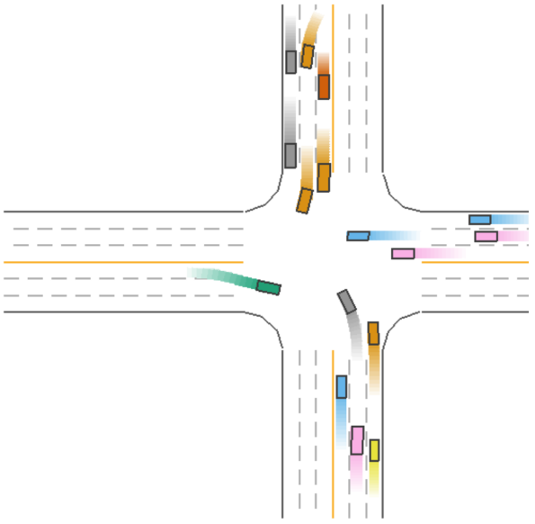
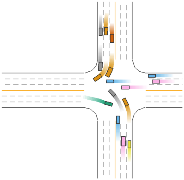
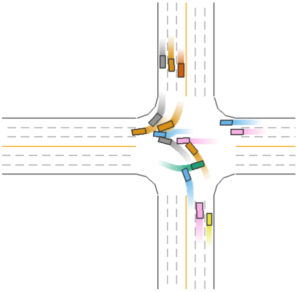
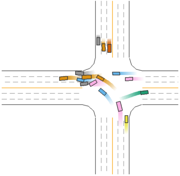
Figure 5: Driving Process of Model 5 (Green Car) in a Straight Scenario.

As seen in Figure 5, Model 5 (green car) strikes a balance between safety and efficiency during straight driving, ensuring both efficient driving and the ability to avoid collisions.

The driving process for Model 5 (green car) during a left-turn scenario is shown in Figure 6.

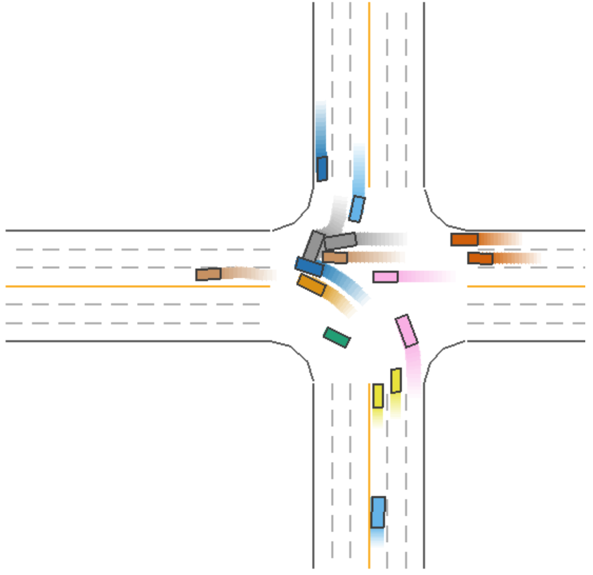
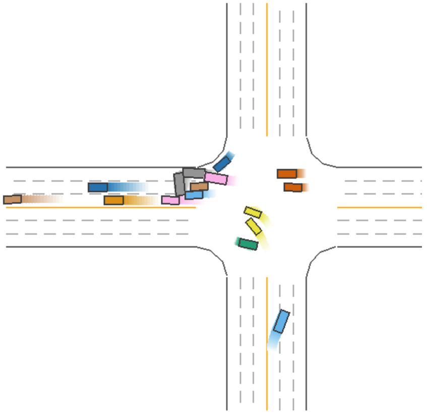
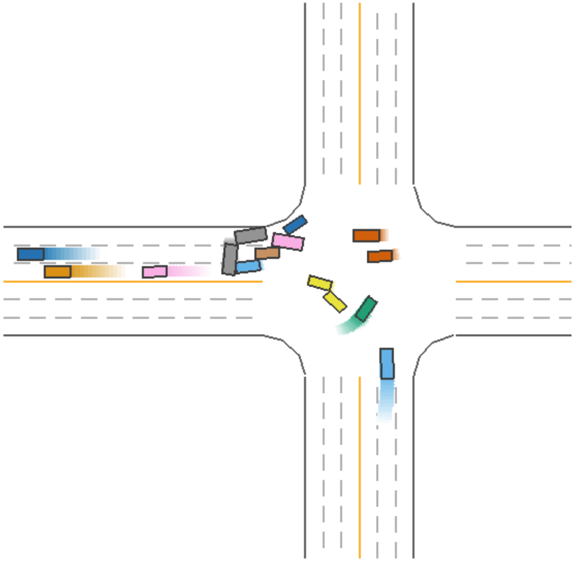
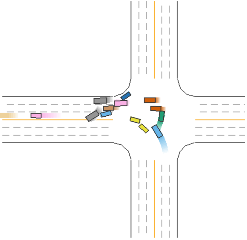
Figure 6: Driving Process of Model 5 (Green Car) in a Left-Turn Scenario.

In Figure 6, we observe that Model 5 (green car) collides during a left turn, despite sacrificing efficiency by waiting. This indicates that, even with safety measures in place, collisions may still occur under certain conditions.

In summary, Model 5 performs best overall, balancing safety and efficiency during right turns and straight driving, though left turns require further optimization. Across all models, success rates during left turns are low, indicating a need for targeted optimization of lateral control rewards. Fixed penalties have limitations; although high fixed penalties improve safety, they drastically reduce efficiency. Low fixed penalties fail to effectively prevent collisions, limiting their practical applicability. Dynamic penalties are better suited for complex interactions, as high-speed collisions incur higher penalties, better reflecting actual risks.

5. Conclusion

5.1. Summary

This paper addresses the challenge of balancing safety and efficiency in autonomous driving by proposing a multi-objective reward function design method based on reinforcement learning. It focuses on developing an effective reward structure and trains seven models with different collision penalty strategies in the MetaDrive simulation environment using the PPO algorithm. Through the collaborative design of wrong-way driving penalties, forward distance rewards, speed rewards, and dynamic/fixed collision penalties, we evaluate the models based on their success rate and average frames required for completion in different turning scenarios. The paper explores the impact of different penalty strategies on driving behavior and seeks to determine the optimal strategy for achieving safe and efficient driving behavior.

Experimental results indicate that models with dynamic collision penalties outperform those with fixed penalties in balancing safety and efficiency. In particular, Model 5 demonstrates the best overall balance in right-turn and straight driving scenarios, optimizing both safety (higher success rate) and efficiency (fewer frames). However, all models show low success rates in left-turn scenarios, highlighting the need for further improvements to the reward structure, especially in lateral control. While fixed penalties effectively improve safety, they significantly reduce efficiency, revealing the limitations of this approach in complex, dynamic environments.

5.2. Addressed Problems

This study addresses the core challenge of multi-objective optimization in autonomous driving by emphasizing the importance of multi-objective optimization and the interplay between safety and efficiency in reward function design. By using dynamic penalty mechanisms (such as speed-related penalties), the study successfully balances safety and efficiency, avoiding the conservative or risky behaviors caused by fixed penalties. This research deepens the understanding of how reinforcement learning can be applied to autonomous driving systems to balance often conflicting objectives. The dynamic reward function's effectiveness in complex interaction scenarios is validated, providing empirical support for multi-objective reinforcement learning. A quantifiable evaluation system based on success rate and frame count was also designed to support multi-scenario, multi-metric analysis of autonomous driving strategies.

5.3. Future Prospects

Although this study has made significant progress in balancing safety and efficiency, there are still areas that require improvement. As previously mentioned, all models perform poorly in left-turn scenarios, indicating the need for more refined lateral control rewards to better handle the unique challenges posed by sharp turns and narrow spaces. Furthermore, expanding the research to include a broader range of traffic scenarios, such as pedestrian interactions, real-time dynamic traffic, and complex weather conditions, would provide a more comprehensive evaluation of the model's robustness in diverse environments.

In the future, my goal is to explore advanced reward shaping techniques, such as hierarchical reinforcement learning, which could better address the long-term dependencies in driving tasks. Additionally, by introducing cognitive architecture or multi-agent systems, incorporating human-like decision-making processes into the model could further enhance its navigation capabilities in dynamic, real-world traffic scenarios. Finally, applying these methods to real-world data and integrating them with current vehicle control systems will be crucial for evaluating their practicality and scalability in real-world autonomous driving applications.

In conclusion, developing reward functions for autonomous driving using reinforcement learning is a complex and multifaceted challenge. This study provides valuable insights into balancing safety and efficiency, and I hope future research will build upon these findings to create safer and more efficient autonomous driving systems.

References

[1]. Russell, S. J., & Norvig, P. (2021). Artificial intelligence: a modern approach, 4th US ed. University of California, Berkeley.
[2]. Bansal, M., Krizhevsky, A., & Ogale, A. (2018). Chauffeurnet: Learning to drive by imitating the best and synthesizing the worst. arXiv preprint arXiv:1812.03079.
[3]. Geiger, A., Lenz, P., Stiller, C., & Urtasun, R. (2013). Vision meets robotics: The kitti dataset. The International Journal of Robotics Research, 32(11), 1231-1237.
[4]. Schwarting, W., Pierson, A., Alonso-Mora, J., Karaman, S., & Rus, D. (2019). Social behavior for autonomous vehicles. Proceedings of the National Academy of Sciences, 116(50), 24972-24978.
[5]. Kong, J., Pfeiffer, M., Schildbach, G., & Borrelli, F. (2015, June). Kinematic and dynamic vehicle models for autonomous driving control design. In 2015 IEEE intelligent vehicles symposium (IV) (pp. 1094-1099). IEEE.
[6]. Kiran, B. R., Sobh, I., Talpaert, V., Mannion, P., Al Sallab, A. A., Yogamani, S., & Pérez, P. (2021). Deep reinforcement learning for autonomous driving: A survey. IEEE Transactions on Intelligent Transportation Systems, 23(6), 4909-4926.
[7]. HAMMA, R., & BOUMARAF, M. (2023). Applying Deep Reinforcement Learning for Autonomous Driving in CARLA Simulator (Doctoral dissertation).
[8]. Lowe, R., Wu, Y. I., Tamar, A., Harb, J., Pieter Abbeel, O., & Mordatch, I. (2017). Multi-agent actor-critic for mixed cooperative-competitive environments. Advances in neural information processing systems, 30.
[9]. Haarnoja, T., Zhou, A., Abbeel, P., & Levine, S. (2018, July). Soft actor-critic: Off-policy maximum entropy deep reinforcement learning with a stochastic actor. In International conference on machine learning (pp. 1861-1870). PMLR.
[10]. Andrychowicz, M., Wolski, F., Ray, A., Schneider, J., Fong, R., Welinder, P., ... & Zaremba, W. (2017). Hindsight experience replay. Advances in neural information processing systems, 30.
[11]. Ng, A. Y., Harada, D., & Russell, S. (1999, June). Policy invariance under reward transformations: Theory and application to reward shaping. In Icml (Vol. 99, pp. 278-287).
[12]. Shalev-Shwartz, S. (2017). On a formal model of safe and scalable self-driving cars. arXiv preprint arXiv:1708.06374.
[13]. Taubman-Ben-Ari, O., Mikulincer, M., & Gillath, O. (2004). The multidimensional driving style inventory—scale construct and validation. Accident Analysis & Prevention, 36(3), 323-332.
[14]. Ziegler, J., Bender, P., Schreiber, M., Lategahn, H., Strauss, T., Stiller, C., ... & Zeeb, E. (2014). Making bertha drive—an autonomous journey on a historic route. IEEE Intelligent transportation systems magazine, 6(2), 8-20.
[15]. Bojarski, M. (2016). End to end learning for self-driving cars. arXiv preprint arXiv:1604.07316.
[16]. Ohn-Bar, E., Prakash, A., Behl, A., Chitta, K., & Geiger, A. (2020). Learning situational driving. In Proceedings of the IEEE/CVF Conference on Computer Vision and Pattern Recognition (pp. 11296-11305).
Cite this article
Zhang,W. (2025). Design of Reward Functions for Autonomous Driving Based on Reinforcement Learning: Balancing Safety and Efficiency. Applied and Computational Engineering,146,9-22.
Data availability
The datasets used and/or analyzed during the current study will be available from the authors upon reasonable request.
Disclaimer/Publisher's Note
The statements, opinions and data contained in all publications are solely those of the individual author(s) and contributor(s) and not of EWA Publishing and/or the editor(s). EWA Publishing and/or the editor(s) disclaim responsibility for any injury to people or property resulting from any ideas, methods, instructions or products referred to in the content.
About volume
Volume title: Proceedings of SEML 2025 Symposium: Machine Learning Theory and Applications
© 2024 by the author(s). Licensee EWA Publishing, Oxford, UK. This article is an open access article distributed under the terms and
conditions of the Creative Commons Attribution (CC BY) license. Authors who
publish this series agree to the following terms:
1. Authors retain copyright and grant the series right of first publication with the work simultaneously licensed under a Creative Commons
Attribution License that allows others to share the work with an acknowledgment of the work's authorship and initial publication in this
series.
2. Authors are able to enter into separate, additional contractual arrangements for the non-exclusive distribution of the series's published
version of the work (e.g., post it to an institutional repository or publish it in a book), with an acknowledgment of its initial
publication in this series.
3. Authors are permitted and encouraged to post their work online (e.g., in institutional repositories or on their website) prior to and
during the submission process, as it can lead to productive exchanges, as well as earlier and greater citation of published work (See
Open access policy for details).